


 这篇博客介绍了如何使用Python和数学原理详细地从头开始构建神经网络,适合初学者理解神经网络的工作原理。
python神经网络代码
机器学习 , 学术 , 教程 (Machine Learning, Scholarly, Tutorial)
Author(s): Pratik Shukla, Roberto Iriondo
作者:Pratik Shukla,Roberto Iriondo
Last updated, June 29, 2020
上次更新时间:2020年6月29日
Note: In our second tutorial on neural networks, we dive in-depth on the limitations and advantages of using neural networks. We show how to implement neural nets with hidden layers and how these lead to a higher accuracy rate on our predictions, along with implementation samples in Python on Google Colab.
注意: 在第二篇 有关神经网络的教程中 ,我们深入探讨了使用神经网络的局限性和优势。 我们将展示如何使用隐藏层实现神经网络,以及如何在我们的预测中提高隐藏率,以及Google Colab中Python的实现示例。

什么是神经网络? (What is a neural network?)
Neural networks form the base of deep learning, which is a subfield of machine learning, where the structure of the human brain inspires the algorithms. Neural networks take input data, train themselves to recognize patterns found in the data, and then predict the output for a new set of similar data. Therefore, a neural network can be thought of as the functional unit of deep learning, which mimics the behavior of the human brain to solve complex data-driven problems.
神经网络构成了深度学习的基础,深度学习是机器学习的一个子领域,人脑的结构在此启发着算法。 神经网络获取输入数据,训练自己以识别数据中发现的模式,然后预测一组新的相似数据的输出。 因此,可以将神经网络视为深度学习的功能单元,它模仿人脑的行为来解决复杂的数据驱动问题。
The first thing that comes to our mind when we think of “neural networks” is biology, and indeed, neural nets are inspired by our brains.
当我们想到“ 神经网络 ”时,我们想到的第一件事就是生物学,而事实上,神经网络是由我们的大脑激发的。
Let’s try to understand them:
让我们尝试了解它们:
![Figure 2: An image representing a biological neuron | Source: Wikipedia [1]](https://i-blog.csdnimg.cn/blog_migrate/700aedc9c7721a2405640591913293e5.png)
In machine learning, the neurons’ dendrites refer to as input, and the nucleus process the data and forward the calculated output through the axon. In a biological neural network, the width (thickness) of dendrites defines the weight associated with it.
在机器学习中,神经元的树突称为输入,原子核处理数据并通过轴突转发计算出的输出。 在生物神经网络中,树突的宽度(厚度)定义了与之相关的重量。
指数: (Index:)
Case Study: Predicting Virus Contraction with a Neural Net with Python
1.什么是人工神经网络? (1. What is an Artificial Neural Network?)
Simply put, an ANN represents interconnected input and output units in which each connection has an associated weight. During the learning phase, the network learns by adjusting these weights in order to be able to predict the correct class for input data.
简而言之,ANN代表互连的输入和输出单元,其中每个连接都具有关联的权重。 在学习阶段,网络通过调整这些权重进行学习,以便能够预测输入数据的正确类别。
For instance:
例如:
We encounter ourselves in a deep sleep state, and suddenly our environment starts to tremble. Immediately afterward, our brain recognizes that it is an earthquake. At once, we think of what is most valuable to us:
我们陷入深度睡眠状态,突然我们的环境开始颤抖。 之后,我们的大脑立即意识到这是地震。 我们立刻想到了对我们最有价值的东西:
- Our beloved ones. 亲爱的
- Essential documents. 基本文件。
- Jewelry. 首饰。
- Laptop. 笔记本电脑。
- A pencil. 铅笔。
Now we only have a few minutes to get out of the house, and we can only save a few things. What will our priorities be in this case?
现在,我们只有几分钟的时间才能出门,而且我们只能保存一些东西。 在这种情况下,我们的优先事项是什么?
Perhaps, we are going to save our beloved ones first, and then if time permits, we can think of other things. What we did here is, we assigned a weight to our valuables. Each of the valuables at that moment is an input, and the priorities are the weights we assigned it to it.
也许,我们将首先拯救我们心爱的人,然后,如果时间允许,我们可以考虑其他事情。 我们在这里所做的是,我们为贵重物品分配了重量。 那时的每种贵重物品都是输入,而优先级是我们为其分配的权重。
The same is the case with neural networks. We assign weights to different values and predict the output from them. However, in this case, we do not know the associated weight with each input, so we make an algorithm that will calculate the weights associated with them by processing lots of input data.
神经网络也是如此。 我们将权重分配给不同的值,并预测它们的输出。 但是,在这种情况下,我们不知道每个输入的关联权重,因此我们制定了一种算法,该算法将通过处理大量输入数据来计算与它们关联的权重。
2.人工神经网络的应用: (2. Applications of Artificial Neural Networks:)
一个。 数据分类: (a. Classification of data:)
Based on a set of data, our trained neural network predicts whether it is a dog or a cat?
根据一组数据,我们训练有素的神经网络可以预测是狗还是猫?
b。 异常检测: (b. Anomaly detection:)
Given the details about transactions of a person, it can say that whether the transaction is fraud or not.
给定有关一个人的交易的详细信息,它可以说该交易是否为欺诈。
C。 语音识别: (c. Speech recognition:)
We can train our neural network to recognize speech patterns. Example: Siri, Alexa, Google assistant.
我们可以训练神经网络来识别语音模式。 示例:Siri,Alexa,Google助手。
d。 音频生成: (d. Audio generation:)
Given the inputs as audio files, it can generate new music based on various factors like genre, singer, and others.
给定输入作为音频文件,它可以根据各种因素(例如流派,歌手和其他因素)生成新音乐。
e。 时间序列分析: (e. Time series analysis:)
A well trained neural network can predict the stock price.
训练有素的神经网络可以预测股票价格。
F。 拼写检查: (f. Spell checking:)
We can train a neural network that detects misspelled spellings and can also suggest a similar meaning for words. Example: Grammarly
我们可以训练一个神经网络来检测拼写错误的拼写,也可以为单词提供类似的含义。 示例:语法
G。 字符识别: (g. Character recognition:)
A well trained neural network can detect handwritten characters.
训练有素的神经网络可以检测手写字符。
H。 机器翻译: (h. Machine translation:)
We can develop a neural network that translates one language into another language.
我们可以开发一种神经网络,将一种语言翻译成另一种语言。
一世。 图像处理: (i. Image processing:)
We can train a neural network to process an image and extract pieces of information from it.
我们可以训练神经网络来处理图像并从中提取信息。
3.人工神经网络(ANN)的一般结构: (3. General Structure of an Artificial Neural Network (ANN):)


4.什么是感知器? (4. What is a Perceptron?)
A perceptron is a neural network without any hidden layer. A perceptron only has an input layer and an output layer.
感知器是没有任何隐藏层的神经网络。 感知器仅具有输入层和输出层。

我们在哪里可以使用感知器? (Where we can use perceptrons?)
Perceptrons’ use lies in many case scenarios. While a perceptron is mostly used for simple decision making, these can also come together in larger computer programs to solve more complex problems.
感知器的使用存在于许多情况下。 虽然感知器通常用于简单的决策,但是它们也可以在较大的计算机程序中结合使用,以解决更复杂的问题。
For instance:
例如:
- Give access if a person is a faculty member and deny access if a person is a student. 如果某人是教师,则授予访问权限;如果某人是学生,则拒绝访问。
- Provide entry for humans only. 仅允许人类进入。
Implementation of logic gates [2].
逻辑门的实现[ 2 ]。
实施神经网络涉及的步骤: (Steps involved in the implementation of a neural network:)
A neural network executes in 2 steps :
神经网络执行两个步骤:
1.前馈: (1. Feedforward:)
On a feedforward neural network, we have a set of input features and some random weights. Notice that in this case, we are taking random weights that we will optimize using backward propagation.
在前馈神经网络上,我们具有一组输入特征和一些随机权重。 请注意,在这种情况下,我们采用随机权重,将使用反向传播对其进行优化。
2.反向传播: (2. Backpropagation:)
During backpropagation, we calculate the error between predicted output and target output and then use an algorithm (gradient descent) to update the weight values.
在反向传播期间,我们计算预测输出和目标输出之间的误差,然后使用算法(梯度下降)更新权重值。
为什么我们需要反向传播? (Why do we need backpropagation?)
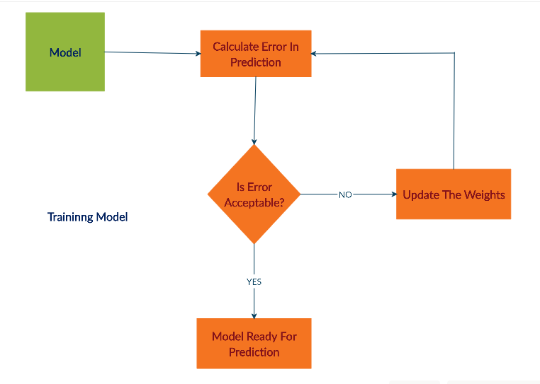
While designing a neural network, first, we need to train a model and assign specific weights to each of those inputs. That weight decides how vital is that feature for our prediction. The higher the weight, the greater the importance. However, initially, we do not know the specific weight required by those inputs. So what we do is, we assign some random weight to our inputs, and our model calculates the error in prediction. Thereafter, we update our weight values and rerun the code (backpropagation). After individual iterations, we can get lower error values and higher accuracy.
在设计神经网络时,首先,我们需要训练模型并为每个输入分配特定的权重。 权重决定了该功能对于我们的预测有多重要。 重量越高,重要性就越大。 但是,最初,我们不知道这些输入所需的具体权重。 所以我们要做的是,为输入分配一些随机权重,然后我们的模型计算预测误差。 此后,我们更新体重值并重新运行代码(反向传播)。 经过单独的迭代,我们可以获得更低的误差值和更高的精度。
总结人工神经网络: (Summarizing an Artificial Neural Network:)
- Take inputs 接受输入
- Add bias (if required) 添加偏见(如果需要)
- Assign random weights to input features 为输入要素分配随机权重
- Run the code for training. 运行代码进行培训。
- Find the error in prediction. 查找预测中的错误。
- Update the weight by gradient descent algorithm. 通过梯度下降算法更新权重。
- Repeat the training phase with updated weights. 使用更新的权重重复训练阶段。
- Make predictions. 作出预测。
一个简单的神经网络流程图: (Flow chart for a simple neural network:)

神经网络的训练阶段: (The training phase of a neural network:)
5. Perceptron示例: (5. Perceptron Example:)
Below is a simple perceptron model with four inputs and one output.
以下是具有四个输入和一个输出的简单感知器模型。


What we have here is the input values and their corresponding target output values. So what we are going to do, is assign some weight to the inputs and then calculate their predicted output values.
我们这里是输入值及其对应的目标输出值。 因此,我们要做的是为输入分配一些权重,然后计算其预测的输出值。
In this example we are going to calculate the output by the following formula:
在此示例中,我们将通过以下公式计算输出:

For the sake of this example, we are going to take the bias value = 0 for simplicity of calculation.
出于本示例的考虑,为了简化计算,我们将偏倚值= 0。
a. Let’s take W = 3 and check the predicted output.
一个。 让我们取W = 3并检查预测输出。

b. After we have found the value of predicted output for W=3, we are going to compare it with our target output, and by doing that, we can find the error in the prediction model. Keep in mind that our goal is to achieve minimum error and maximum accuracy for our model.
b。 在找到W = 3的预测输出值之后,我们将其与目标输出进行比较,然后,可以在预测模型中找到误差。 请记住,我们的目标是实现模型的最小误差和最大准确性。

c. Notice that in the above calculation, there is an error in 3 out of 4 predictions. So we have to change the parameter values of our weight to set in low. Now we have two options:
C。 请注意,在上述计算中,在4个预测中有3个存在误差。 因此,我们必须将重量的参数值更改为低值。 现在我们有两个选择:
- Increase weight 增加体重
- Decrease weight 减轻体重
First, we are going to increase the value of the weight and check whether it leads to a higher error rate or lower error rate. Here we increased the weight value by 1 and changed it to W = 4.
首先,我们将增加权重的值,并检查它是导致更高的错误率还是更低的错误率。 在这里,我们将权重值增加了1,并将其更改为W = 4。

d. As we can see in the figure above, is that the error in prediction is increasing. So now we can conclude that increasing the weight value does not help us in reducing the error in prediction.
d。 如上图所示,预测误差正在增加。 因此,现在我们可以得出结论,增加权重值并不能帮助我们减少预测误差。

e. After we fail in increasing the weight value, we are going to decrease the value of weight for it. Furthermore, by doing that, we can see whether it helps or not.
e。 在无法增加权重值之后,我们将为其降低权重值。 此外,通过这样做,我们可以看到它是否有帮助。

f. Calculate the error in prediction. Here we can see that we have achieved the global minimum.
F。 计算预测中的误差。 在这里我们可以看到我们已经达到了全球最低要求。

In figure 17, we can see that there is no error in prediction.
在图17中,我们可以看到预测中没有错误。
Now what we did here:
现在我们在这里做了什么:
- First, we have our input values and target output. 首先,我们有输入值和目标输出。
- Then we initialized some random value to W, and then we proceed further. 然后我们将一些随机值初始化为W,然后继续进行。
- Last, we calculated the error for in prediction for that weight value. Afterward, we updated the weight and predicted the output. After several trial and error epochs, we can reduce the error in prediction. 最后,我们针对该权重值计算了预测误差。 之后,我们更新了权重并预测了输出。 经过几次反复试验后,我们可以减少预测中的误差。
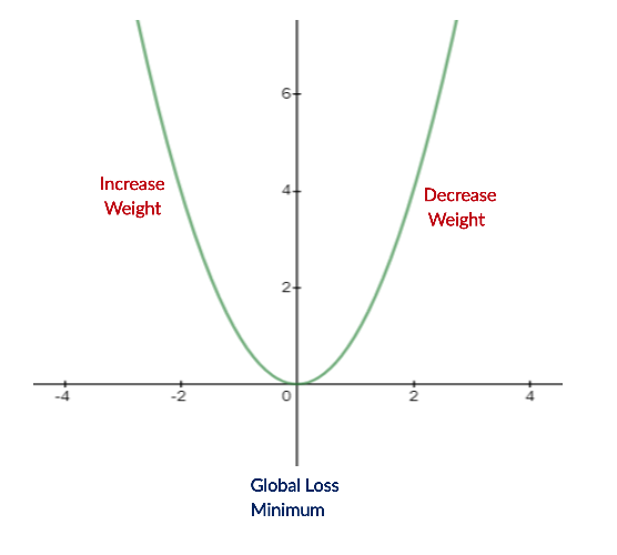
So, we are trying to get the value of weight such that the error becomes minimum. We need to figure out whether we need to increase or decrease the weight value. Once we know that, we keep on updating the weight value in that direction until error becomes minimum. We might reach a point where if further updates occur to the weight, the error will increase. At that time, we need to stop, and that is our final weight value.
因此,我们正在尝试获得权重值,以使误差最小。 我们需要弄清楚是否需要增加或减少重量值。 一旦知道了这一点,我们将继续在该方向上更新权重值,直到误差最小为止。 如果权重发生进一步的更新,误差可能会增加。 那时,我们需要停下来,这就是我们最终的体重值。
In real-life data, the situation can be a bit more complex. In the example above, we saw that we could try different weight values and get the minimum error manually. However, in real-life data, weight values are often decimal (non-integer). Therefore, we are going to use a gradient descent algorithm with a low learning rate so that we can try different weight values and obtain the best predictions from our model.
在实际数据中,情况可能会更加复杂。 在上面的示例中,我们看到可以尝试不同的权重值并手动获得最小误差。 但是,在实际数据中,权重值通常是十进制(非整数)。 因此,我们将使用学习率较低的梯度下降算法,以便我们可以尝试不同的权重值并从模型中获得最佳预测。

6.乙状结肠功能: (6. Sigmoid Function:)
A sigmoid function serves as an activation function in our neural network training. We generally use neural networks for classifications. In binary classification, we have 2 types. However, as we can see, our output value can be any possible number from the equation we used. To solve that problem, we use a sigmoid function. Now for classification, we want our output values to be 0 or 1. So to get values between 0 and 1 we use the sigmoid function. The sigmoid function converts our output values between 0 and 1.
乙状结肠功能在我们的神经网络训练中充当激活功能 。 我们通常使用神经网络进行分类。 在二进制分类中,我们有2种类型。 但是,正如我们所看到的,我们的输出值可以是我们使用的公式中的任何可能的数字。 为了解决这个问题,我们使用了S形函数。 现在进行分类,我们希望我们的输出值为0或1。因此,要使用0到1之间的值,请使用Sigmoid函数。 sigmoid函数可在0到1之间转换我们的输出值。
Let’s have a look at it:
让我们看一下:

Let’s visualize our sigmoid function with Python:
让我们用Python可视化Sigmoid函数:

Output:
输出:

Explanation:
说明:
In figure 21 and 22, for any input values, the value of the sigmoid function will always lie between 0 and 1. Here notice that for negative numbers, the output of the sigmoid function is ≤0.5, or we can say closer to zero, and for positive numbers, the output is going to be >0.5, or we can say closer to 1.
在图21和22中,对于任何输入值,S形函数的值将始终位于0到1之间。这里请注意,对于负数,S形函数的输出为≤0.5,或者我们可以说接近于零,对于正数,输出将> 0.5,或者我们可以说接近1。
7.从零开始的神经网络实现: (7. Neural Network Implementation from Scratch:)
We are going to do is implement the “OR” logic gate using a perceptron. Keep in mind that here we are not going to use any of the hidden layers.
我们要做的是使用感知器实现“或”逻辑门。 请记住,这里我们将不使用任何隐藏层。
什么是逻辑或门? (What is logical OR Gate?)
Straightforwardly, when one of the inputs is 1, the output of the OR gate is going to be 1. It means that the output is 0 only when both of the inputs are 0.
直接地,当输入之一为1时,或门的输出将为1。这意味着仅当两个输入均为0时,输出才为0。
表示: (Representation:)

或门的真值表: (Truth-Table for OR gate:)

或门的感知器: (Perceptron for the OR gate:)

Next, we are going to assign some weights to each of the input values and calculate it.
接下来,我们将为每个输入值分配一些权重并进行计算。

示例:(手动计算) (Example: (Calculating Manually))
a. Calculate the input for o1:
一个。 计算o1的输入:

b. Calculate the output value:
b。 计算输出值:


Notice that from our truth table, we can see that we wanted the output of 1, but what we get here is 0.68997. Now we need to calculate the error and then backpropagate and then update the weight values.
注意,从真值表中,我们可以看到我们想要的输出为1,但这里得到的是0.68997。 现在我们需要计算误差,然后反向传播,然后更新权重值。
c. Error Calculation:
C。 误差计算:
Next, we are going to use Mean Squared Error for calculating the error :
接下来,我们将使用均方误差来计算误差:

The summation sign (Sigma symbol) means that we have to add our error for all our input sets. Here we are going to see how that works for only one input set.
求和符号(Sigma符号)意味着我们必须为所有输入集添加误差。 在这里,我们将看到它仅对一个输入集起作用。

We have to do the same for all the remaining inputs. Now that we have found the error, we have to update the values of weight to make the error minimum. For updating weight values, we are going to use a gradient descent algorithm.
我们必须对所有其余输入执行相同的操作。 现在我们已经找到了错误,我们必须更新权重值以使错误最小。 为了更新权重值,我们将使用梯度下降算法。
8.什么是梯度下降? (8. What is Gradient Descent?)
Gradient Descent is a machine learning algorithm that operates iteratively to find the optimal values for its parameters. It takes into account, user-defined learning rate, and initial parameter values.
梯度下降是一种机器学习算法,可迭代运行以找到其参数的最佳值。 它考虑了用户定义的学习率和初始参数值。
Working: (Iterative)
工作:(迭代)
1. Start with initial values.
1.从初始值开始。
2. Calculate cost.
2.计算成本。
3. Update values using the update function.
3.使用更新功能更新值。
4. Returns minimized cost for our cost function
4.为我们的成本函数返回最小成本
我们为什么需要它? (Why do we need it?)
Generally, what we do is, we find the formula that gives us the optimal values for our parameter. However, in this algorithm, it finds the value by itself!
通常,我们要做的是找到可以为我们的参数提供最佳值的公式。 但是,在此算法中,它会自行查找值!
Interesting, isn’t it?
有趣,不是吗?

We are going to update our weight with this algorithm. First of all, we need to find the derivative f(X).
我们将使用此算法更新权重。 首先,我们需要找到导数f(X)。
9.推导神经网络中使用的公式 (9. Derivation of the formula used in a neural network)
Next, what we want to find is how a particular weight value affects the error. To find that we are going to apply the chain rule.
接下来,我们要查找的是特定重量值如何影响误差。 发现我们将应用链式规则。

Afterward, what we have to do is we have to find values for these three derivatives.
之后,我们要做的就是找到这三个导数的值。
In the following images, we have tried to show the derivation of each of these derivatives to showcase the math behind gradient descent.
在以下图像中,我们试图显示这些导数中的每一个的派生,以展示梯度下降背后的数学原理。
d. Calculating derivatives:
d。 计算导数:

In our case:
在我们的情况下:
Output = 0.68997Target = 1
输出= 0.68997目标= 1

e. Finding the second part of the derivative:
e。 找到导数的第二部分:

To understand it step-by-step:
要逐步了解它,请执行以下操作:
e.a. Value of outo1:
ea out1的值:

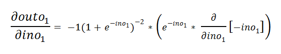
e.b. Finding the derivative with respect to ino1:
eb找到关于ino1的导数:

e.c. Simplifying it a bit to find the derivative easily:
ec稍微简化一下即可轻松找到导数:

e.d. Applying chain rule and power rule:
ed应用链规则和幂规则:

e.e. Applying sum rule:
ee应用求和规则:

e.f. The derivative of constant is zero:
ef常数的导数为零:

e.g. Applying exponential rule and chain rule:
例如,应用指数规则和链式规则:
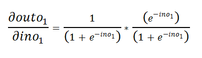
e.h. Simplifying it a bit:
eh简化一下:

e.i. Multiplying both negative signs:
ei将两个负号相乘:

e.j. Put the negative power in the denominator:
ej将负幂设为分母:

That is it. However, we need to simplify it as it is a little complex for our machine learning algorithm to process for a large number of inputs.
这就对了。 但是,我们需要简化它,因为对于我们的机器学习算法而言,要处理大量输入会有点复杂。
e.k. Simplifying it:
ek简化它:

e.l. Further simplification:
el进一步简化:
e.k. Adding +1–1:
ek加+ 1–1:

e.l. Separate the parts:
el分离各部分:

e.m. Simplify:
简化:

e.n. Now we all know the value of outo1 from equation 1:
现在我们都从等式1知道outo1的值:

e.o. From that we can derive the following final derivative:
eo由此,我们可以得出以下最终导数:

e.p. Calculating the value of our input:
ep计算输入值:

f. Finding the third part of the derivative :
F。 找到导数的第三部分:

f.a Value of ino:
fa ino 值 :

f.b. Finding derivative:
fb查找导数:
All the other values except w2 will be considered constant here.
除w2以外的所有其他值在这里都将视为常量。

f.c Calculating both values for our input:
fc计算输入的两个值:

f.d. Putting it all together:
fd全部放在一起:

f.e. Putting it in our main equation:
fe把它放在我们的主要方程式中:

f.f. We can calculate:
ff我们可以计算:

Notice that the value of the weight has increased here. We can calculate all the values in this way, but as we can see, it is going to be a lengthy process. So now we are going to implement all the steps in Python.
请注意,此处的权重值已增加。 我们可以通过这种方式计算所有值,但是正如我们所看到的,这将是一个漫长的过程。 因此,现在我们将在Python中实现所有步骤。
人工实施神经网络的摘要: (Summary of The Manual Implementation of a Neural Network:)

a. Input for perceptron:
一个。 感知器输入:

b. Applying sigmoid function for predicted output :
b。 将Sigmoid函数应用于预测输出:

c. Calculate the error:
C。 计算误差:

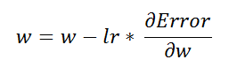
d. Changing the weight value based on gradient descent formula:
d。 根据梯度下降公式更改权重值:
e. Calculating the derivative:
e。 计算导数:

f. Individual derivatives:
F。 个别衍生产品:

Source: Image created by the author.
资料来源:作者创作的图片。

Source: Image created by the author.
资料来源:作者创作的图片。

g. After then we run the same code with updated weight values.
G。 之后,我们使用更新的权重值运行相同的代码。
Let’s code:
让我们编写代码:
10.用Python实现神经网络: (10. Implementation of a Neural Network In Python:)
10.1导入所需的库: (10.1 Import Required libraries:)
First, we are going to import Python libraries. We are using NumPy for the calculations:
首先,我们将导入Python库。 我们使用NumPy进行计算:

10.2分配输入值: (10.2 Assign Input values:)
Next, we are going to take input values for which we want to train our neural network. Here we can see that we have taken two input features. In actual data sets, the value of the input features is mostly high.
接下来,我们将采用我们要为其训练神经网络的输入值。 在这里我们可以看到我们采用了两个输入功能。 在实际数据集中,输入要素的值通常很高。

10.3目标输出: (10.3 Target Output:)
For the input features, we want to have a specific output for specific input features. It is called the target output. We are going to train the model that gives us the target output for our input features.
对于输入要素,我们希望有针对特定输入要素的特定输出。 它称为目标输出。 我们将训练模型,该模型为我们的输入功能提供目标输出。

10.3分配权重: (10.3 Assign the Weights :)
Next, we are going to assign random weights to the input features. Note that our model is going to modify these weight values to be optimum. At this point, we are taking these values randomly. Here we have two input features, so we are going to take two weight values.
接下来,我们将为输入要素分配随机权重。 请注意,我们的模型将修改这些权重值以使其最佳。 此时,我们正在随机获取这些值。 这里我们有两个输入功能,因此我们将采用两个权重值。

10.4添加偏差值和分配学习率: (10.4 Adding Bias Values and Assigning a Learning Rate :)
Now here we are going to add the bias value. The value of bias = 1. However, the weight assigned to it is random at first, and our model will optimize it for our target output.
现在在这里,我们将添加偏差值。 bias的值=1。但是,分配给它的权重最初是随机的,我们的模型将针对目标输出对其进行优化。
The other parameter is called the learning rate(LR). We are going to use the learning rate in a gradient descent algorithm to update the weight values. Generally, we keep the learning rate as low as possible so that we can achieve a minimum error rate.
另一个参数称为学习率(LR)。 我们将在梯度下降算法中使用学习率来更新权重值。 通常,我们将学习率保持在尽可能低的水平,以便可以实现最小的错误率。

10.5应用S形函数: (10.5 Applying a Sigmoid Function:)
Once we have our weight values and input features, we are going to send it to the main function that predicts the output. Now notice that our input features and weight values can be anything, but here we want to classify data, so we need the output between 0 and 1. For such, we are going to a sigmoid function.
一旦我们有了权重值和输入特征,就将其发送给预测输出的主要功能。 现在注意,我们的输入特征和权重值可以是任何值,但是这里我们要对数据进行分类,因此我们需要0到1之间的输出。为此,我们将使用S型函数。

10.6 S型函数的导数: (10.6 Derivative of sigmoid function:)
In gradient descent algorithm we are going to need the derivative of the sigmoid function.
在梯度下降算法中,我们将需要S型函数的导数。

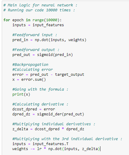
10.7预测输出和更新重量值的主要逻辑: (10.7 The main logic for predicting output and updating the weight values:)
We are going to explain the following code step-by-step.
我们将逐步解释以下代码。

它是如何工作的? (How does it work?)
First of all, the code above will need to run approximately 10,000 times. Keep in mind that if we only run this code a few times, then probably we are going to have a higher error rate. Therefore, in short, we can say that we are going to update the weight values 10,000 times to reach the optimal value possible.
首先,上面的代码将需要运行大约10,000次。 请记住,如果我们只运行几次此代码,则可能会有更高的错误率。 因此,简而言之,可以说我们将权重值更新10,000次以达到可能的最佳值。
Next, what we need to do is multiply the input features with it is corresponding weight values, the values we are going to feed to the perceptron can be represented in the form of a matrix.
接下来,我们需要做的是将输入要素乘以对应的权重值,然后将要馈入感知器的值以矩阵的形式表示。
in_o represents the dot product of input_features and weight. Notice that the first matrix (input features) is of size (4*2), and the second matrix (weights) is of size (2*1). After multiplication, the resultant matrix is of size (4*1).
in_o表示input_features和weight的点积。 请注意,第一个矩阵(输入要素)的大小为(4 * 2),第二个矩阵(权重)的大小为(2 * 1)。 乘法之后,所得矩阵的大小为(4 * 1)。

In the above representation, each of those boxes represents a value.
在上面的表示中,每个框代表一个值。
Now in our formula, we also have the bias value. Let’s understand it with simple matrix representation.
现在在我们的公式中,我们还有偏差值。 让我们用简单的矩阵表示来了解它。

Next, we are going to add the bias value. Addition operation in the matrix is easy to understand. Such is the input for the sigmoid function. Afterward, we are going to apply the sigmoid function to our input value, which will give us the predicted output value between 0 and 1.
接下来,我们将添加偏差值。 矩阵中的加法运算很容易理解。 这就是S形函数的输入。 之后,我们将对输入值应用S型函数,这将为我们提供0到1之间的预测输出值。
Next, we have to calculate the error in prediction. We generally use Mean Squared Error (MSE) for this, but here we are just going to use simple error function for simplicity in the calculation. Last, we are going to add the error for all of our four inputs.
接下来,我们必须计算预测误差。 我们通常为此使用均方误差(MSE) ,但是在这里,为了简化计算,我们将仅使用简单误差函数。 最后,我们将为所有四个输入添加错误。
Our ultimate goal is to minimize the error. To minimize the error, we can update the value of our weights. To update the weight value, we are going to use a gradient descent algorithm.
我们的最终目标是最大程度地减少错误。 为了使误差最小,我们可以更新权重的值。 要更新权重值,我们将使用梯度下降算法。
To find the derivative, we are going to need the values of some derivatives for our gradient descent algorithm. As we have already discussed, we are going to find 3 individual values for derivatives and then multiply it.
为了找到导数,我们将需要一些用于梯度下降算法的导数的值。 正如我们已经讨论的那样,我们将为导数找到3个单独的值,然后将其相乘。
The first derivative is:
一阶导数是:

The second derivative is:
二阶导数是:

The third derivative is:
三阶导数是:

Notice that we can easily find the values of the first two derivatives as they are not dependent on inputs. Next, we store the values of the multiplication of the first two derivatives in the deriv variable. Now the values of these derivatives must be of the same size as the size of weights. The size of the weights is (2*1).
注意,我们可以轻松地找到前两个导数的值,因为它们不依赖于输入。 接下来,我们存储在所述第一两种衍生物的相乘的值deriv变量。 现在,这些导数的值必须与权重的大小相同。 权重的大小为(2 * 1)。
To find the final derivative, we need to find the transpose of our input_features and then we are going to multiply it with our deriv variable that is basically the multiplication of the other two derivatives.
为了找到最终的衍生,我们需要找到我们的转置input_features ,然后我们会用我们的相乘deriv变量,基本上是其他两种衍生品的乘法。
Let’s have a look at the matrix representation of the operation.
让我们看一下操作的矩阵表示。

On figure 83, the first matrix is the transposed matrix of input_features. The second matrix stores the values of the multiplication of the other two derivatives. Now see that we have stored these values in a matrix called deriv_final. Notice that, the size of deriv_final is (2*1) which is the same as the size of our weight matrix (2*1).
在图83上,第一个矩阵是input_features的转置矩阵。 第二个矩阵存储其他两个导数相乘的值。 现在看到我们已经将这些值存储在名为deriv_final的矩阵中。 注意, deriv_final的大小为(2 * 1),与我们的权重矩阵(2 * 1)的大小相同。
Afterward, we update the weight value, notice that we have all the values needed for updating our weight. We are going to use the following formula to update the weight values.
然后,我们更新权重值,请注意,我们拥有更新权重所需的所有值。 我们将使用以下公式更新重量值。

Last, we need to update the bias value. If we remember the diagram, we might have noticed that the value of bias weight is not dependent on the input. So we have to update it separately. In this case, we need the deriv values, as it is not dependent on the input values. To update the bias value, we go through the for loop for updating value at each input on every iteration.
最后,我们需要更新偏差值。 如果我们记住该图,可能已经注意到偏差权重的值不取决于输入。 因此,我们必须单独更新它。 在这种情况下,我们需要deriv值,因为它不依赖于输入值。 为了更新偏差值,我们通过for循环来更新每次迭代中每个输入的值。
10.8检查权重和偏差的值: (10.8 Check the Values of Weight and Bias:)

On figure 85, notice that our weight and bias values have changed from our randomly assigned values.
在图85上,请注意,我们的权重和偏差值已与我们随机分配的值发生了变化。
10.9 Predicting values :
10.9预测值:
Since we have trained our model, we can start to make predictions from it.
由于我们已经训练了模型,因此可以开始从中进行预测。
10.9.1 Prediction for (1,0):
10.9.1(1,0)的预测:
Target value = 1
目标值= 1

On figure 86, we can see the predicted output is very near to 1.
在图86上,我们可以看到预测的输出非常接近1。
10.9.2 Prediction for (1,1):
10.9.2(1,1)的预测:
Target output = 1
目标输出= 1

On figure 87, we can see that the predicted output is very close to 1.
在图87上,我们可以看到预测的输出非常接近1。
10.9.3 Prediction for (0,0):
10.9.3(0,0)的预测:
Target output = 0
目标输出= 0

On figure 88, we can see that the predicted output is very close to 0.
在图88上,我们可以看到预测的输出非常接近0。
放在一起: (Putting it all together:)
# Import required libraries:
import numpy as np# Define input features:
input_features = np.array([[0,0],[0,1],[1,0],[1,1]])
print (input_features.shape)
print (input_features)# Define target output:target_output = np.array([[0,1,1,1]])# Reshaping our target output into vector:
target_output = target_output.reshape(4,1)
print(target_output.shape)
print (target_output)# Define weights:
weights = np.array([[0.1],[0.2]])
print(weights.shape)
print (weights)# Bias weight:
bias = 0.3# Learning Rate:
lr = 0.05# Sigmoid function:
def sigmoid(x):
return 1/(1+np.exp(-x))# Derivative of sigmoid function:
def sigmoid_der(x):
return sigmoid(x)*(1-sigmoid(x))# Main logic for neural network:# Running our code 10000 times:for epoch in range(10000):
inputs = input_features#Feedforward input:
in_o = np.dot(inputs, weights) + bias #Feedforward output:
out_o = sigmoid(in_o) #Backpropogation#Calculating error
error = out_o - target_output#Going with the formula:
x = error.sum()
print(x)#Calculating derivative:
derror_douto = error
douto_dino = sigmoid_der(out_o)#Multiplying individual derivatives:
deriv = derror_douto * douto_dino #Multiplying with the 3rd individual derivative:
#Finding the transpose of input_features:
inputs = input_features.T
deriv_final = np.dot(inputs,deriv)#Updating the weights values:
weights -= lr * deriv_final #Updating the bias weight value:
for i in deriv:
 bias -= lr * i #Check the final values for weight and biasprint (weights)print (bias) #Taking inputs:
single_point = np.array([1,0]) #1st step:
result1 = np.dot(single_point, weights) + bias #2nd step:
result2 = sigmoid(result1) #Print final result
print(result2) #Taking inputs:
single_point = np.array([1,1]) #1st step:
result1 = np.dot(single_point, weights) + bias #2nd step:
result2 = sigmoid(result1) #Print final result
print(result2) #Taking inputs:
single_point = np.array([0,0]) #1st step:
result1 = np.dot(single_point, weights) + bias #2nd step:
result2 = sigmoid(result1) #Print final result
print(result2)
Launch it on Google Colab:
在Google Colab上启动它:
为什么我们要增加偏见? (Why do we add bias?)
Suppose if we have input values (0,0), the sum of the products of the input nodes and weights is always going to be zero. In this case, the output will always be zero, no matter how much we train our model. To resolve this issue and make reliable predictions, we use the bias term. In short, we can say that the bias term is necessary to make a robust neural network.
假设我们有输入值(0,0),则输入节点与权重的乘积之和始终为零。 在这种情况下,无论我们训练模型多少,输出都将始终为零。 为了解决此问题并做出可靠的预测,我们使用偏差项。 简而言之,我们可以说偏置项对于构建鲁棒的神经网络是必不可少的。
Therefore, how does the value of bias affects the shape of our sigmoid function? Let’s visualize it with some examples.
因此, 偏差值如何影响我们的S型函数的形状? 让我们通过一些示例对其进行可视化。
To change the steepness of the sigmoid curve, we can adjust the weight accordingly.
要更改S型曲线的陡度,我们可以相应地调整权重。
For instance:
例如:


From the output, we can quickly notice that for negative values, the output of the sigmoid function is going to be ≤0.5. Moreover, for positive values, the output is going to be >0.5.
从输出中,我们可以很快注意到,对于负值,S型函数的输出将≤0.5。 此外,对于正值,输出将> 0.5。
From the figure (red curve), you can see that if we decrease the value of the weight, it decreases the value of steepness, and if we increase the value of weight (green curve), it increases the value of steepness. However, for all of the three curves, if the input is negative, the output is always going to be ≤0.5. For positive numbers, the output is always going to be >0.5.
从图中(红色曲线),您可以看到,如果减小权重的值,则减小陡度的值;如果增大权重的值(绿色曲线),则增大陡度的值。 但是,对于所有三个曲线,如果输入为负,则输出将始终≤0.5。 对于正数,输出始终将> 0.5。
如果我们想改变这种模式怎么办? (What if we want to change this pattern?)
For such case scenarios, we use bias values.
对于这种情况,我们使用偏差值。


From the output, we can notice that we can shift the curves on the x-axis that helps us to change the pattern we show in the previous example.
从输出中,我们可以注意到我们可以移动x轴上的曲线,这有助于我们更改上一个示例中显示的模式。
摘要: (Summary:)

In neural networks:
在神经网络中:
- We can view bias as a threshold value for activation. 我们可以将偏差视为激活的阈值。
- Bias increases the flexibility of the model 偏差增加了模型的灵活性
- The bias value allows us to shift the activation function to the right or left. 偏置值使我们可以将激活函数向右或向左移动。
- The bias value is most useful when we have all zeros (0,0) as input. 当我们将所有零(0,0)作为输入时,偏置值最有用。
Let’s try to understand it with the same example we saw earlier. Nevertheless, here we are not going to add the bias value. After the model has trained, we will try to predict the value of (0,0). Ideally, it should be close to zero. Now let’s check out the following example.
让我们尝试使用我们之前看到的相同示例来理解它。 不过,这里我们将不添加偏差值。 训练模型后,我们将尝试预测(0,0)的值。 理想情况下,它应该接近零。 现在,让我们看看下面的示例。
没有偏差值的实现: (An Implementation Without Bias Value:)
一个。 导入所需的库: (a. Import required libraries:)

b。 输入功能: (b. Input features:)

C。 目标输出: (c. Target output:)

d。 定义输入权重: (d. Define Input weights:)

e。 定义学习率: (e. Define the learning rate:)

F。 激活功能: (f. Activation function:)

G。 S型函数的导数: (g. A derivative of the sigmoid function:)

H。 训练模型的主要逻辑: (h. The main logic for training our model:)
Here notice that we are not going to use bias values anywhere.
在这里请注意,我们不会在任何地方使用偏差值。
一世。 做出预测: (i. Making predictions:)
i.a. Prediction for (1,0) :
ia(1,0)的预测:
Target output = 1
目标输出= 1

From the predicted output we can see that it’s close to 1.
从预测的输出中,我们可以看到它接近1。
i.b. Prediction for (0,0) :
ib对(0,0)的预测:
Target output = 0
目标输出= 0
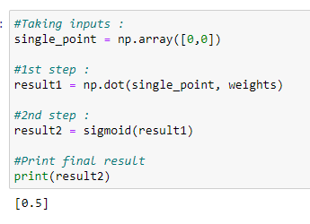
Here we can see that it’s nowhere near 0. So we can say that our model failed to predict it. This is the reason for adding the bias value.
在这里,我们可以看到它离0不远。因此,可以说我们的模型无法对其进行预测。 这就是添加偏差值的原因。
i.c. Prediction for (1,1):
(1,1)的ic预测:
Target output = 1
目标输出= 1

We can see that it’s close to 1.
我们可以看到它接近1。
放在一起: (Putting it all together:)
# Import required libraries :
import numpy as np# Define input features :
input_features = np.array([[0,0],[0,1],[1,0],[1,1]])
print (input_features.shape)
print (input_features)# Define target output :
target_output = np.array([[0,1,1,1]])# Reshaping our target output into vector :
target_output = target_output.reshape(4,1)
print(target_output.shape)
print (target_output)# Define weights :
weights = np.array([[0.1],[0.2]])
print(weights.shape)
print (weights)# Define learning rate :
lr = 0.05# Sigmoid function :
def sigmoid(x):
 return 1/(1+np.exp(-x))# Derivative of sigmoid function :
def sigmoid_der(x):
 return sigmoid(x)*(1-sigmoid(x))# Main logic for neural network :
# Running our code 10000 times :for epoch in range(10000):
 inputs = input_features#Feedforward input :
 pred_in = np.dot(inputs, weights)#Feedforward output :
 pred_out = sigmoid(pred_in)#Backpropogation
 #Calculating error
 error = pred_out — target_output
 x = error.sum()
 #Going with the formula :
 print(x)
 #Calculating derivative :
 dcost_dpred = error
 dpred_dz = sigmoid_der(pred_out)
 #Multiplying individual derivatives :
 z_delta = dcost_dpred * dpred_dz#Multiplying with the 3rd individual derivative :
 inputs = input_features.T
 weights -= lr * np.dot(inputs, z_delta)
#Taking inputs :
single_point = np.array([1,0])#1st step :
result1 = np.dot(single_point, weights)#2nd step :
result2 = sigmoid(result1)#Print final result
print(result2)#Taking inputs :
single_point = np.array([0,0])#1st step :
result1 = np.dot(single_point, weights)#2nd step :
result2 = sigmoid(result1)#Print final result
print(result2)#Taking inputs :
single_point = np.array([1,1])#1st step :
result1 = np.dot(single_point, weights)#2nd step :
result2 = sigmoid(result1)#Print final result
print(result2)📚 Check out an overview of machine learning algorithms for beginners with code examples in Python 📚
with通过Python代码示例,为初学者学习机器学习算法的概述📚
案例研究:使用Python用神经网络预测病毒收缩 (Case Study: Predicting Virus Contraction with a Neural Net with Python)

资料集: (Dataset:)
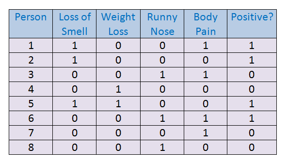
For this example, our goal is to predict whether a person is positive for a virus or not based on the given input features. Here 1 represents “Yes” and 0 represents “No”.
对于此示例,我们的目标是根据给定的输入特征来预测某个人的病毒阳性。 这里1代表“是”,0代表“否”。
Let’s code:
让我们编写代码:
一个。 导入所需的库: (a. Import required libraries:)

Source: Image created by the author.
资料来源:作者创作的图片。
b。 输入功能: (b. Input features:)

C。 目标输出: (c. Target output:)

d。 定义权重: (d. Define weights:)

e。 偏差值和学习率: (e. Bias value and learning rate:)

F。 乙状结肠功能: (f. Sigmoid function:)

G。 S型函数的导数: (g. Derivative of sigmoid function:)

H。 训练模型的主要逻辑: (h. The main logic for training model:)

一世。 做出预测: (i. Making predictions:)
i.a. A tested person is positive for the virus.
ia测试对象对该病毒呈阳性。

i.b. A tested person is negative for the virus.
ib被测人对该病毒呈阴性。

i.c. A tested person is positive for the virus.
ic经测试的人对该病毒呈阳性。

j。 最终权重和偏差值: (j. Final weight and bias values:)

In this example, we can notice that the input feature “loss of smell” influences the output the most. If it is true, then in most of the case, the person tests positive for the virus. We can also derive this conclusion from the weight values. Keep in mind that the higher the value of the weight, the more the influence on the output. The input feature “Weight loss” is not affecting the output much, so we can rule it out while we are making predictions for a larger dataset.
在此示例中,我们可以注意到输入特征“气味消失”对输出的影响最大。 如果属实,那么在大多数情况下,此人对该病毒的测试呈阳性。 我们还可以从权重值得出此结论。 请记住,权重值越高,对输出的影响越大。 输入特征“失重”对输出的影响不大,因此可以在为更大的数据集进行预测时将其排除。
放在一起: (Putting it all together:)
# Import required libraries :
import numpy as np# Define input features :
input_features = np.array([[1,0,0,1],[1,0,0,0],[0,0,1,1],
 [0,1,0,0],[1,1,0,0],[0,0,1,1],
 [0,0,0,1],[0,0,1,0]])
print (input_features.shape)
print (input_features)# Define target output :
target_output = np.array([[1,1,0,0,1,1,0,0]])# Reshaping our target output into vector :
target_output = target_output.reshape(8,1)
print(target_output.shape)
print (target_output)# Define weights :
weights = np.array([[0.1],[0.2],[0.3],[0.4]])
print(weights.shape)
print (weights)# Bias weight :
bias = 0.3# Learning Rate :
lr = 0.05# Sigmoid function :
def sigmoid(x):
 return 1/(1+np.exp(-x))# Derivative of sigmoid function :
def sigmoid_der(x):
 return sigmoid(x)*(1-sigmoid(x))# Main logic for neural network :
# Running our code 10000 times :for epoch in range(10000):
 inputs = input_features#Feedforward input :
 pred_in = np.dot(inputs, weights) + bias#Feedforward output :
 pred_out = sigmoid(pred_in)#Backpropogation
 #Calculating error
 error = pred_out — target_output
 #Going with the formula :
 x = error.sum()
 print(x)
 #Calculating derivative :
 dcost_dpred = error
 dpred_dz = sigmoid_der(pred_out)
 #Multiplying individual derivatives :
 z_delta = dcost_dpred * dpred_dz#Multiplying with the 3rd individual derivative :
 inputs = input_features.T
 weights -= lr * np.dot(inputs, z_delta)#Updating the bias weight value :
 for i in z_delta:
  bias -= lr * i#Printing final weights: print (weights)
print (“\n\n”)
print (bias)#Taking inputs :
single_point = np.array([1,0,0,1])#1st step :
result1 = np.dot(single_point, weights) + bias#2nd step :
result2 = sigmoid(result1)#Print final result
print(result2)#Taking inputs :
single_point = np.array([0,0,1,0])#1st step :
result1 = np.dot(single_point, weights) + bias#2nd step :
result2 = sigmoid(result1)#Print final result
print(result2)#Taking inputs :
single_point = np.array([1,0,1,0])#1st step :
result1 = np.dot(single_point, weights) + bias#2nd step :
result2 = sigmoid(result1)#Print final result
print(result2)
Launch it on Google Colab:
在Google Colab上启动它:
In the examples above, we did not use any hidden layers for calculations. Notice that in the above examples, our data were linearly separable. For instance:
在上面的示例中,我们没有使用任何隐藏层进行计算。 注意,在以上示例中,我们的数据是线性可分离的。 例如:


We can see that the red line can separate the yellow dots (value = 1) and green dot (value = 0 ).
We can see that the red line can separate the yellow dots (value = 1) and green dot (value = 0 ).
Limitations of a Perceptron Model (Without Hidden Layers): (Limitations of a Perceptron Model (Without Hidden Layers):)
1. Single-layer perceptrons cannot classify non-linearly separable data points.
1. Single-layer perceptrons cannot classify non-linearly separable data points.
2. Complex problems that involve many parameters do not resolve with single-layer perceptrons.
2. Complex problems that involve many parameters do not resolve with single-layer perceptrons.
However, in several cases, the data is not linearly separable. In that case, our perceptron model (without hidden layers) fails to make accurate predictions. To make accurate predictions, we need to add one or more hidden layers.Visual representation of non-linearly separable data:
However, in several cases, the data is not linearly separable. In that case, our perceptron model (without hidden layers) fails to make accurate predictions. To make accurate predictions, we need to add one or more hidden layers.Visual representation of non-linearly separable data:

DISCLAIMER: The views expressed in this article are those of the author(s) and do not represent the views of Carnegie Mellon University, nor other companies (directly or indirectly) associated with the author(s). These writings do not intend to be final products, yet rather a reflection of current thinking, along with being a catalyst for discussion and improvement.
DISCLAIMER: The views expressed in this article are those of the author(s) and do not represent the views of Carnegie Mellon University, nor other companies (directly or indirectly) associated with the author(s). These writings do not intend to be final products, yet rather a reflection of current thinking, along with being a catalyst for discussion and improvement.
Published via Towards AI
Published via Towards AI
Recommended Articles (Recommended Articles)
I. Best Datasets for Machine Learning and Data ScienceII. AI Salaries Heading SkywardIII. What is Machine Learning?IV. Best Masters Programs in Machine Learning (ML) for 2020V. Best Ph.D. Programs in Machine Learning (ML) for 2020VI. Best Machine Learning BlogsVII. Key Machine Learning DefinitionsVIII. Breaking Captcha with Machine Learning in 0.05 SecondsIX. Machine Learning vs. AI and their Important DifferencesX. Ensuring Success Starting a Career in Machine Learning (ML)XI. Machine Learning Algorithms for BeginnersXII. Neural Networks from Scratch with Python Code and Math in DetailXIII. Building Neural Networks with PythonXIV. Main Types of Neural NetworksXV. Monte Carlo Simulation Tutorial with PythonXVI. Natural Language Processing Tutorial with Python
I. Best Datasets for Machine Learning and Data Science II. AI Salaries Heading Skyward III. What is Machine Learning? IV。 Best Masters Programs in Machine Learning (ML) for 2020 V. Best Ph.D. Programs in Machine Learning (ML) for 2020 VI. Best Machine Learning Blogs VII. Key Machine Learning Definitions VIII. Breaking Captcha with Machine Learning in 0.05 Seconds IX. Machine Learning vs. AI and their Important Differences X. Ensuring Success Starting a Career in Machine Learning (ML) XI. Machine Learning Algorithms for Beginners XII. Neural Networks from Scratch with Python Code and Math in Detail XIII. Building Neural Networks with Python XIV. Main Types of Neural Networks XV. Monte Carlo Simulation Tutorial with Python XVI. Natural Language Processing Tutorial with Python
引文 (Citation)
For attribution in academic contexts, please cite this work as:
For attribution in academic contexts, please cite this work as:
Shukla, et al., “Neural Networks from Scratch with Python Code and Math in Detail — I”, Towards AI, 2020BibTex citation: (BibTex citation:)
@article{pratik_iriondo_2020,
 title={Neural Networks from Scratch with Python Code and Math in Detail — I},
 url={https://towardsai.net/neural-networks-with-python},
 journal={Towards AI},
 publisher={Towards AI Co.},
 author={Pratik, Shukla and Iriondo,
 Roberto},
 year={2020},
 month={Jun}
}python神经网络代码


 2165
2165

 被折叠的 条评论
为什么被折叠?
被折叠的 条评论
为什么被折叠?
 到【灌水乐园】发言


