机器学习:梯度下降_从零开始的机器学习：分类，回归，聚类和梯度下降

weixin_26726011

于 2020-08-21 02:00:53 发布

阅读量643

点赞数

文章标签：机器学习深度学习逻辑回归人工智能 python

原文链接：https://medium.com/swlh/machine-learning-101-classification-regression-gradient-descent-and-clustering-b3449f270dbe

版权

机器学习:梯度下降

A quick start “from scratch” on 3 basic machine learning models — Linear regression, Logistic regression, K-means clustering, and Gradient Descent, the optimisation algorithm acting as a driving force behind them.

快速入门从3种基本机器学习模型开始-线性回归，逻辑回归，K-均值聚类和梯度下降，优化算法是它们背后的驱动力。

The purpose of this article is for coders to understand the inner workings of basic machine learning algorithms. To make the best use of the article, it is recommended to follow the code on your own development environment to understand the process.

本文的目的是让编码人员了解基本机器学习算法的内部工作原理。为了充分利用本文，建议您在自己的开发环境中遵循代码以理解该过程。

线性回归 (Linear Regression)

Linear regression models a linear relationship between an independent variable X and a continuous dependent variable y. Linear regression is an example of supervised learning, the task of learning a function mapping given X and y. A continuous variable can take any value within an interval (e.g. 0.01, 1.23), while a discrete variable can only take distinct and separate values (e.g. 0, 1). Discrete variables will be addressed in the later section on Logistic Regression.

线性回归建模自变量X和连续因变量y之间的线性关系。线性回归是监督学习的一个示例，该学习是在给定X和y下学习函数映射的任务。连续变量可以取任何值的时间间隔内(例如0.01 ， 1.23 )，而离散变量只能采取不同的和单独的值(例如0 ， 1 )。离散变量将在后面的Logistic回归中讨论。

A linear model can be simply defined by the following equation, where m and c represents the gradient of the line and the y-intercept respectively.:

线性模型可以通过以下方程式简单定义，其中m和c代表直线和y轴截距的梯度：

y = m*X + c

The gradient and the y-intercept are commonly referred to as the weight and the bias respectively. When X is multi-dimensional, the equation becomes that of a multiple linear regression model:

梯度和y轴截距通常分别称为权重和偏差。当X为多维时，该方程式变为多元线性回归模型的方程式：

y = m1*X1 + m2*X2 + m3*X3 + C

The weights and dependent variables can be represented as vectors m = [m1,m2,m3] and x = [x1,x2,x3]. To consolidate in Python 3.8, the linear regression function for 1-dimensional X can be defined as using list comprehension:

权重和因变量可以表示为向量m = [m1,m2,m3]和x = [x1,x2,x3] 。为了在Python 3.8中进行整合，可以使用列表理解将一维X的线性回归函数定义为：

import numpy as np
import pandas as pd
import matplotlib.pyplot as plt
plt.style.use('seaborn')
import randomdef f(m, X, c):
    """Linear regression"""
    return [m * x + c for x in X]X = [i for i in range(10)]
y = [x + random.random() for x in X]m, c = 1, 0
y_hat = f(m, X, c)plt.plot(X, y, '.', c='r')
plt.plot(X, y_hat)
plt.show()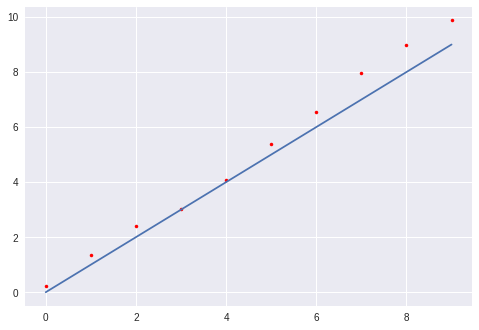

Image for post — Matplotlib plot of linear regression

The linear regression model y = 1 * X + 0 where m = 1 and c = 0 seems to fit the data reasonably well but a quantifiable measure is required in order to compare between models with different values of m and c.

线性回归模型y = 1 * X + 0 ，其中m = 1和c = 0似乎很适合数据，但是需要进行量化的比较，以便在m和c不同的模型之间进行比较。

The error of the model can be quantified in terms of the difference between y, the actual output, and y_hat, the prediction of the model. One error measure is Mean Squared Error, defined as:

可以根据y (实际输出)与y_hat (模型的预测)之间的差来量化模型的误差。一种误差度量是均方误差，定义为：

def MSE(y, y_hat):
    """Mean squared error"""
    c = 0
    n = len(y)
    for i in range(n):
        c += (y_hat[i] - y[i]) ** 2
    return 1/2 * c/nprint(cost(y, y_hat))  # 0.17272072055396498

A lower mean squared error indicates parameters that result in a better-fitting linear regression model. The goal of optimising a model is to minimise the error. Therefore, an optimisation algorithm, such as gradient descent, is required.

均方误差越低，表明导致线性拟合模型拟合度越高的参数。优化模型的目的是使误差最小化。因此，需要优化算法，例如梯度下降。

梯度下降 (Gradient Descent)

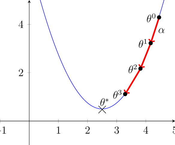
Gradient descent is an optimisation algorithm for finding the local minimum of a differentiable function. The loss function mse = (y_hat - y)**2 of a linear regression model may be minimised to improve model fitness. In the following diagram, the vertical axis represents the MSE while the horizontal-axis represents a weight, e.g. m. By changing the value of m, the MSE may increase or decrease. To minimise MSE, m must move towards a direction where MSE decreases.

梯度下降是一种用于找到可微函数的局部最小值的优化算法。可以最小化线性回归模型的损失函数mse = (y_hat - y)**2 ，以提高模型的适用性。在下图中，垂直轴表示MSE，而水平轴表示权重，例如m 。通过更改m的值，MSE可以增加或减少。为了最小化MSE， m必须朝MSE降低的方向移动。

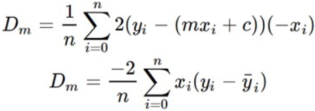
In the case of the above loss function, a positive gradient signals a need to decrease theta and a negative one, increase. The gradient, or partial derivative, of the loss function with respect to m is computed as:

在上述损失函数的情况下，正梯度表示需要减小theta ，负梯度增大。损失函数相对于m的梯度或偏导数的计算公式如下：

The key step in gradient descent is therefore the weight update, where a represents the learning rate, a hyperparameter that controls the size of the change in weight. The bias, c, also changes in the same way. The following is the gradient descent algorithm.

因此，梯度下降的关键步骤是权重更新，其中a表示学习率，是控制权重变化大小的超参数。偏差c也以相同的方式变化。以下是梯度下降算法。

# No. of iterations, weight, bias, learning rate
e, m, c, a = 10, 1, 0, 0.01for i in range(e):
    y_hat = f(m, X, c)
    n = len(y_hat)
    
    # Compute partial derivatives of MSE w.r.t. m and c
    dm = (-2/n) * sum([X[i] * (y[i] - y_hat[i]) for i in range(n)])
    dc = (-2/n) * sum([y[i] - y_hat[i] for i in range(n)])
    
    # Update weight and bias
    m = m - a * dm
    c = c - a * dc
    
    print(f"Epoch {i}: m={m:.2f}, c={c:.2f}")y_hat = f(m, X, c)
plt.plot(X, y, '.', c='r')
plt.plot(X, y_hat)
plt.show()

逻辑回归 (Logistic Regression)

Logistic regression uses a logistic function (or sigmoid function) to model a binary (discrete) dependent variable, usually either 0 and 1. Logistic regression is commonly used for classification tasks, such as predicting if a passenger survives on board the sinking Titanic ship.

Logistic回归使用logistic函数(或Sigmoid函数)来建模二进制( 离散 )因变量，通常为0和1 。 Logistic回归通常用于分类任务，例如预测下沉的泰坦尼克号船上是否有乘客幸存。

The sigmoid function is defined as:

乙状结肠功能定义为：

import mathdef sigmoid(z):
    return 1 / (1 + math.exp(-z))X = [i for i in range(-10,10)]
y = [sigmoid(x) for x in X]
plt.plot(X, y)
plt.show()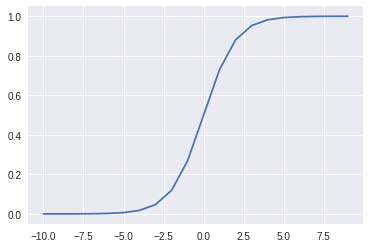

The loss function for logistic regression (“log-loss”) is defined as:

逻辑回归的损失函数(“对数损失”)定义为：

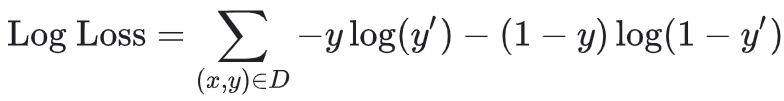
When the actual value of y is 0, the first term -y*log(y_hat) equals 0, and log-loss equals -log(1-y_hat). If y_hat is close to 0, e.g. y_hat=0.1, -log(1–0.1) equals ~0.105, while if y_hat is close to 1, e.g. y_hat=0.9, -log(1-0.9) equals ~2.303, indicating a higher loss when y_hat differs from y greatly.

当y的实际值为0时，第一项-y*log(y_hat)等于0，对数损耗等于-log(1-y_hat) 。如果y_hat接近于0，例如y_hat=0.1 ，则-log(1–0.1)等于-log(1–0.1) ，而如果y_hat接近于1，例如y_hat=0.9 ，则-log(1-0.9)等于-log(1-0.9) ，表示更高y_hat与y相差很大时的损失。

The loss function can be adjusted to become:

损失函数可以调整为：

import mathdef loss(y, y_hat):
    n = len(y)
    loss = 0    for i in range(n):
        loss += -y[i] * math.log(y_hat[i]) - (1-y[i]) * math.log(1-y_hat[i])
    return loss / ny_hat = [sigmoid(x + random.uniform(-1,1)) for x in X]
plt.plot(X, y_hat, label='noisy')
plt.plot(X, y, label='sigmoid')
plt.legend(loc='upper left')
plt.show()
print("Loss:", loss(y, y_hat))  # 0.17083318165128286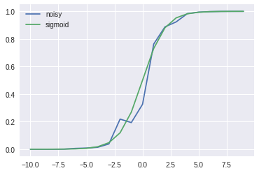

K均值聚类 (K-Means Clustering)

K-Means Clustering is a method of grouping data points together based on similarity between one another, forming clusters. K-means clustering is an unsupervised learning algorithm, requiring only X (data points) without the need for y (cluster index).

K-均值聚类是一种基于彼此之间的相似性将数据点分组在一起的方法，从而形成聚类。 K-均值聚类是一种无监督的学习算法，仅需要X (数据点)，而无需y (集群索引)。

The K-means clustering algorithm is well-explained in words:

K-means聚类算法可以用词来很好地解释：

Randomly initialise K centroids (points).
随机初始化K个质心(点)。
Assign each data point to the closest centroid.
将每个数据点分配给最近的质心。
Compute the mean of all points assigned for each unique centroid, and re-assign the K centroids with the newly computed mean.
计算分配给每个唯一质心的所有点的平均值，然后用新计算的平均值重新分配K质心。
Repeat steps 2–3.
重复步骤2-3。

步骤1：随机初始化K个质心。 (Step 1: Randomly initialise K centroids.)

from sklearn.datasets import make_blobsX, y = make_blobs(n_samples=20, random_state=0)
random.seed(1)# Randomly initialise k=3 centroids
k = 3
centroids = np.array([
    [random.uniform(-5, 5), random.uniform(-5, 5)],
    [random.uniform(-5, 5), random.uniform(-5, 5)],
    [random.uniform(-5, 5), random.uniform(-5, 5)]])plt.scatter(X[:,0], X[:,1])
plt.scatter(centroids[:,0], centroids[:,1], c='r')
plt.show()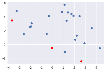

步骤2：将每个数据点分配给最近的质心。 (Step 2: Assign each data point to the closest centroid.)

cluster_labels = []
for x in X:
    dists = []
    for c in centroids:
        # Euclidean distance
        d = math.sqrt((x[0] - c[0])**2 + (x[1] - c[1])**2)
        dists.append(d)
    cluster_labels.append(dists.index(min(dists)))print(cluster_labels)
# [0, 0, 2, 2, 1, 0, 0, 2, 0, 2, 2, 2, 2, 2, 2, 0, 0, 0, 1, 0]

步骤3：计算分配给每个唯一质心的所有点的平均值，然后用新计算的平均值重新分配K质心。 (Step 3: Compute the mean of all points assigned for each unique centroid, and re-assign the K centroids with the newly computed mean.)

# Compute the mean of all points assigned for each unique centroid
new_centroids = []
for i in range(k):
    data_points = []
        for j in range(len(cluster_labels)):
            if cluster_labels[j] == i:
                data_points.append(X[j])
        if len(data_points) == 0:
            new_centroids.append(centroids[i])
        else:
            new_c = sum(data_points)/len(data_points)
            new_centroids.append(new_c)new_centroids = np.array(new_centroids)
print("Centroids:", new_centroids)# Centroids:
[[-0.94637217  3.75181235]
 [ 3.62236293 -0.20060169]
 [ 1.77693338  2.32752122]]cls0_idx = np.where(np.array(cluster_labels)==0)[0]
cls1_idx = np.where(np.array(cluster_labels)==1)[0]
cls2_idx = np.where(np.array(cluster_labels)==2)[0]plt.scatter(X[cls0_idx,0], X[cls0_idx,1], c='yellow')
plt.scatter(X[cls1_idx,0], X[cls1_idx,1], c='blue')
plt.scatter(X[cls2_idx,0], X[cls2_idx,1], c='green')
plt.scatter(new_centroids[:,0], new_centroids[:,1], c='r')
plt.show()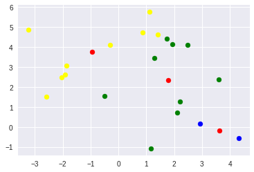

步骤4：重复步骤2-3(在功能中！)。 (Step 4: Repeat steps 2–3 (in a function!).)

def kmeans_clustering(centroids, X):
    """K-means clustering"""
    # Assign each data point to closest centroid
    cluster_labels = []
    
    for x in X:
        dists = []
        for c in centroids:
            # Euclidean distance
            d = math.sqrt((x[0] - c[0])**2 + (x[1] - c[1])**2)
            dists.append(d)
        cluster_labels.append(dists.index(min(dists)))    # Compute the mean of all points assigned as each unique centroid
    new_centroids = []
    for i in range(k):
        data_points = []
        for j in range(len(cluster_labels)):
            if cluster_labels[j] == i:
                data_points.append(X[j])
        if len(data_points) == 0:
            new_centroids.append(centroids[i])
        else:
            new_c = sum(data_points)/len(data_points)
            new_centroids.append(new_c)    new_centroids = np.array(new_centroids)
    return new_centroids, cluster_labels
# Perform 10 iterations of K-means clustering
for i in range(10):
    centroids, cluster_labels = kmeans_clustering(centroids, X)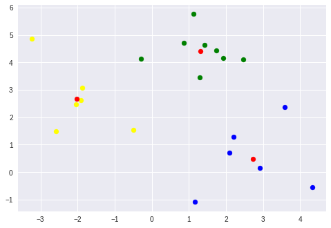

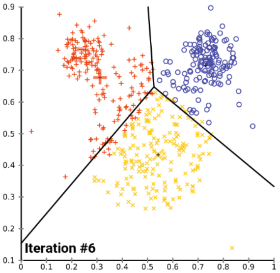
K-means clustering has a hyperparameter k that needs to be specified. If the data has 4 clusters by visual inspection, k=3 will not provide a good clustering of the data.

K均值聚类具有需要指定的超参数k 。如果通过目视检查数据具有4个聚类，则k=3将无法提供良好的数据聚类。

结论 (Conclusion)

This article should provide for you a basic idea and intuition behind machine learning. Each algorithm has its benefits and limitations, so an in-depth inspection of algorithms, beyond a surface-level usage of libraries, provides a deeper understanding of machine learning.

本文应该为您提供机器学习背后的基本思想和直觉。每种算法都有其优点和局限性，因此除了对库的表面用法之外，对算法的深入检查还提供了对机器学习的更深入的了解。

翻译自: https://medium.com/swlh/machine-learning-101-classification-regression-gradient-descent-and-clustering-b3449f270dbe

机器学习:梯度下降

weixin_26726011

关注

0
点赞
踩
1

收藏

觉得还不错? 一键收藏
0
评论
机器学习:梯度下降_从零开始的机器学习：分类，回归，聚类和梯度下降

机器学习:梯度下降A quick start “from scratch” on 3 basic machine learning models — Linear regression, Logistic regression, K-means clustering, and Gradient Descent, the optimisation algorithm acting as a driv...
复制链接

扫一扫