halcon项目实战 灰度投影

一、基本原理

直接上图 灰度投影 顾名思义 也就是一部分区域的投影 如果是水平投影 那就是水平行方向所有灰度值相加再求均值，知道所有行都计算完毕，相同列也是一样。基本理论很简单 如果涉及到所选区域不是对其行列而旋转一定角度。则可以使用插值算法依次计算各个区域的灰度值，再进行该角度方向上的投影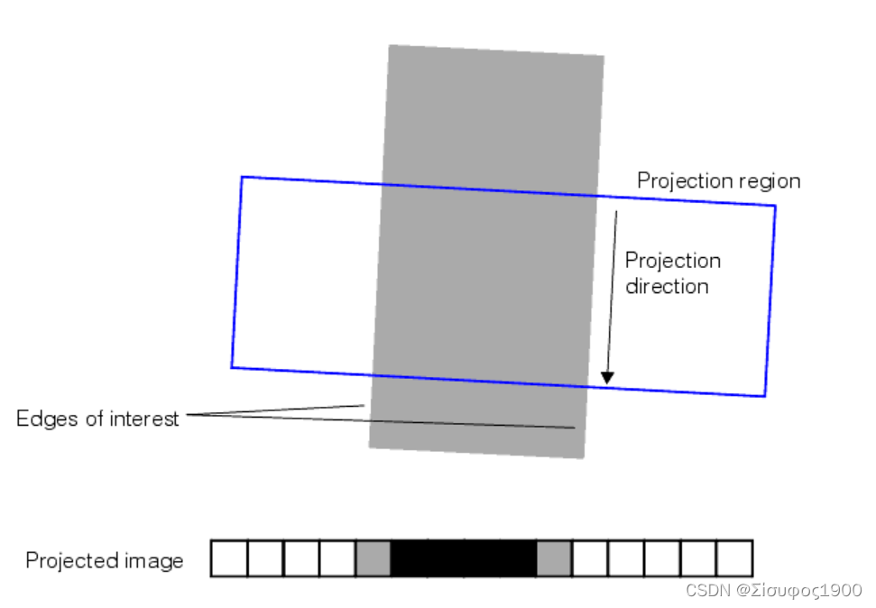

gray,例程,投影,Halcon,灰度,projections 

二、gray_projections算子

halcon特征提取（三）基于统计方式：gray_projections-分类器、神经网络、深度学习-少有人走的路

计算水平和垂直灰度值投影

​
gray_projections(Region, Image : : Mode : HorProjection, VertProjection)
​
** 功能：计算图片在rectangle1区域内的灰度投影
** Region:待处理区域
** image  待投影的灰度图
** Mode = 'simple'，则在图像坐标轴的方向上执行投影
** 输出
** horizontalProjection  水平方向的灰度投影，就是说从
** verticalProjection   竖直方向投影


*如果选择了 Mode = 'simple'，则在图像坐标轴的方向上执行投影，即：

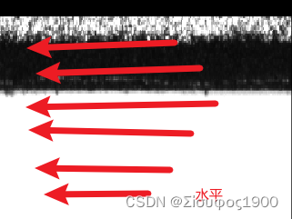
注意：这里的水平和垂直方向的投影

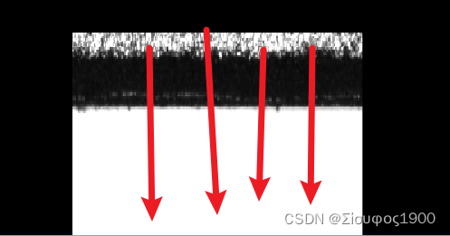
 同理  垂直：

数学原理：

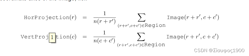
如果选择了 Mode = 'rectangle'，则在输入区域任意方向的最小封闭矩形的主轴方向上执行投影

三、案例

read_image (Image721, 'C:/Users/alber/Desktop/test/721.png')
rgb1_to_gray (Image721, Image721)
get_image_size (Image721, Width2, Height2)

gen_rectangle1 (ROI_0, 103, 11, 202, 360)  // Width=360-11=350   Height=202-103=100
gen_rectangle1 (ROI_1, 23, 11, 222, 360)   // Width1=360-11=350   Height1=202-23=200

reduce_domain (Image721, ROI_0, ImageReduced)
crop_domain (ImageReduced, ImagePart1)

reduce_domain (Image721, ROI_1, ImageReduced3)
crop_domain (ImageReduced3, ImagePart3)

get_image_size (ImagePart1, Width, Height) //350  100
get_image_size (ImagePart3, Width1, Height1) //350 200
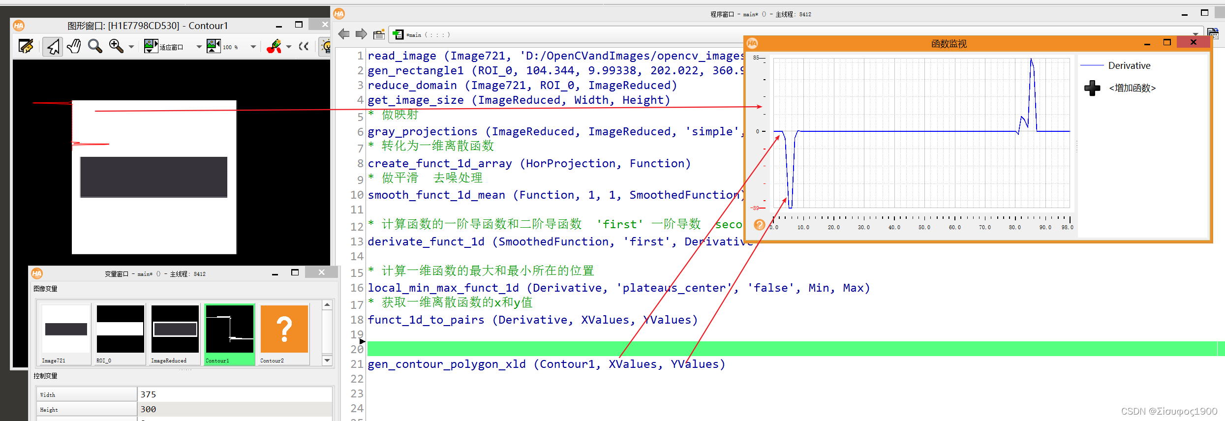
* 做映射
* 得出的结果是 HorProjection 是100 个值  对应的就是高 
* VertProjection 是350个值  对应的就是宽 
* 'simple' 坐标轴
gray_projections (ImageReduced, ImageReduced, 'simple', HorProjection, VertProjection)

* 转化为一维离散函数
create_funct_1d_array (HorProjection, Function)

* 做平滑  去噪处理
* 1 是平滑系数
* 1 是迭代测试
smooth_funct_1d_mean (Function, 1, 1, SmoothedFunction)

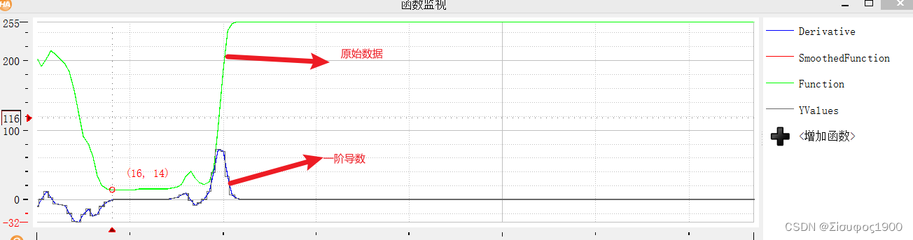
* 计算函数的一阶导函数和二阶导函数  'first' 一阶导数  second是二阶函数
derivate_funct_1d (SmoothedFunction, 'first', Derivative)

* 计算一维函数的最大和最小所在的位置
local_min_max_funct_1d (Derivative, 'plateaus_center', 'false', Min, Max)
* 获取一维离散函数的x和y值
funct_1d_to_pairs (Derivative, XValues, YValues)

gen_contour_polygon_xld (Contour1, XValues, YValues)




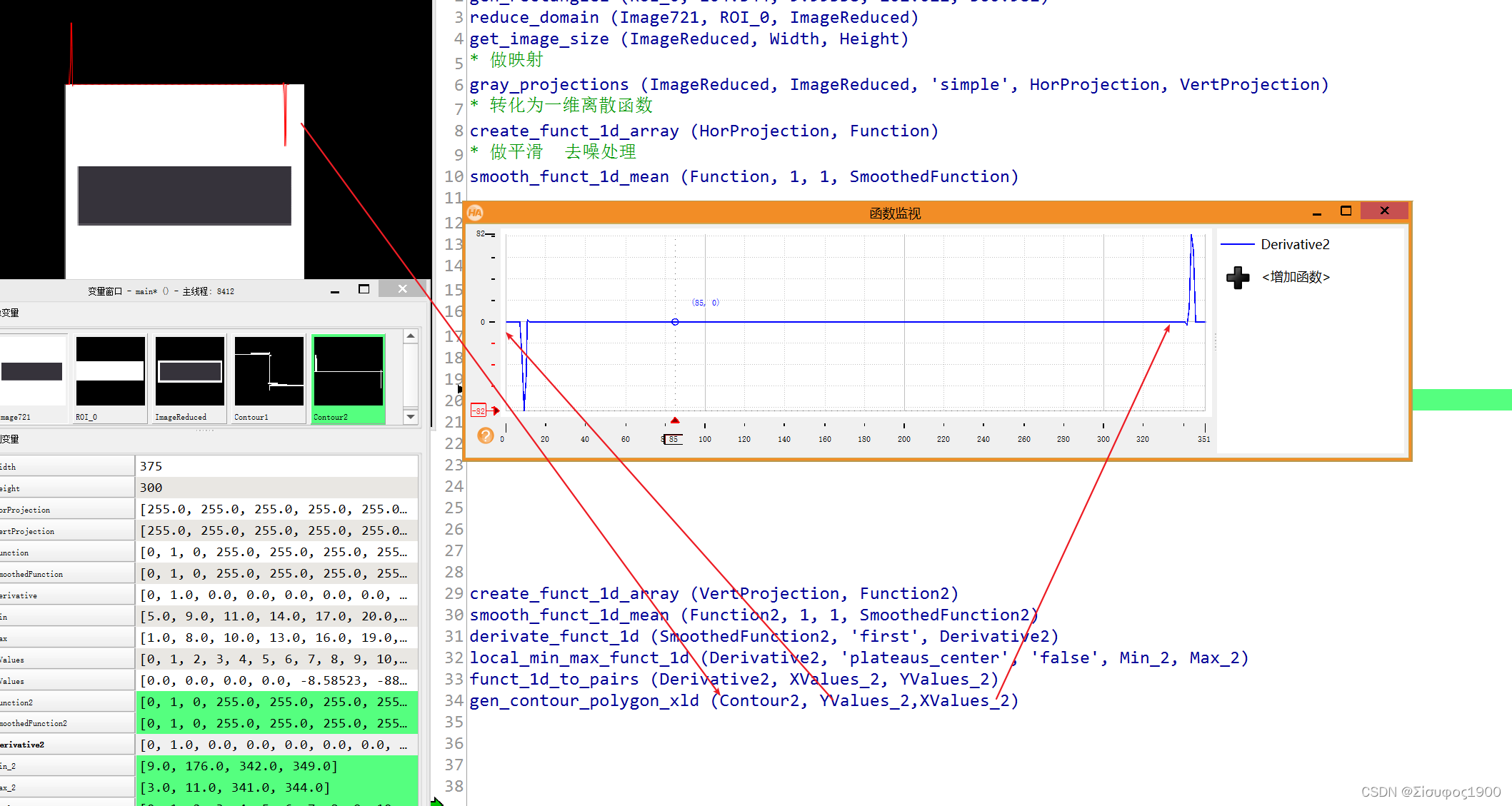
create_funct_1d_array (VertProjection, Function2)
smooth_funct_1d_mean (Function2, 1, 1, SmoothedFunction2)
derivate_funct_1d (SmoothedFunction2, 'first', Derivative2)
local_min_max_funct_1d (Derivative2, 'plateaus_center', 'false', Min_2, Max_2)
funct_1d_to_pairs (Derivative2, XValues_2, YValues_2)
gen_contour_polygon_xld (Contour2, YValues_2,XValues_2)

其中计算一阶导数 和二阶导数 

dev_update_off ()
dev_close_window ()
dev_open_window (0, 0, 512, 512, 'white', WindowHandle)
dev_set_color ('black')
dev_set_line_width (2)
 
X := []
for J := -127 to 128 by 1
    X := [X,J / 20.0]
endfor
tuple_length(X,len)
stop()

* 创建一个（x,y）的函数
create_funct_1d_pairs (X, cos(X), Cos)
 
plot_funct_1d (WindowHandle, Cos, 'x', 'cos(x)', 'red', ['axes_color','origin_x','origin_y'], ['black',0,0])
disp_continue_message (WindowHandle, 'black', 'true')


* 求一介倒数
derivate_funct_1d(Cos,'first', Derivative)
plot_funct_1d (WindowHandle, Derivative, 'x', 'cos(x)', 'blue', ['axes_color','origin_x','origin_y'], ['black',0,0])

derivate_funct_1d(Cos,'second', function_out)
plot_funct_1d (WindowHandle, function_out, 'x', 'cos(x)', 'green', ['axes_color','origin_x','origin_y'], ['black',0,0])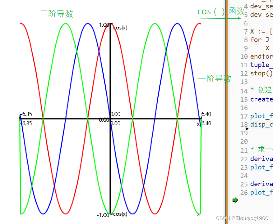

 

案例 

有一个二维码，要识别，但是那个位置飘忽不定，用blob 分析 干扰因素很多 等不稳定，所以用这个方法。可以测试一下

思路就是 在水平和竖直方向分别做投影，计算出起始点和终止点，计算其中心，组合起来，然后进行粗定位

read_image (Image999, 'C:/Users/alber/Desktop/opencv_images/999.png')
rgb1_to_gray (Image999, GrayImage)
get_image_size (GrayImage, Width, Height)
gray_closing_rect (GrayImage, ImageClosing, 15, 15)
* 先灰度投影，然后再计算一阶导数
gray_projections (ImageClosing, ImageClosing, 'simple', HorProjection, VertProjection)
create_funct_1d_array (VertProjection, Function_V)
smooth_funct_1d_mean (Function_V, 1, 1, SmoothedFunction_V)
derivate_funct_1d (SmoothedFunction_V, 'first', Derivative_V)
local_min_max_funct_1d (Derivative_V, 'plateaus_center', 'false', Min, Max)
funct_1d_to_pairs (Derivative_V, XValues, YValues)
derivate_funct_1d (Derivative_V, 'second', Derivative_2s_V)
gen_contour_polygon_xld (Contour1, YValues,XValues)
*拿到最大和最小的队友的坐标位置
startrow:=Max[0]
startowcol:=Height
gen_cross_contour_xld (Cross, startowcol, startrow, 60, 0.785398)
tuple_length (Min, Length)
endrow:=Min[Length-1]
endowcol:=Height
gen_cross_contour_xld (Cross1, endowcol, endrow, 60, 0.785398)

* 计算重点
midcol:=(endrow+startrow)/2
gen_cross_contour_xld (Cross2, endowcol,midcol , 6, 0.785398)