


简 介
Nested CV 提供有助于在生物医学数据中开发和调整机器学习模型的功能,其中样本量通常有限,但预测因子的数量可能要大得多。虽然大多数机器学习管道涉及将数据分成训练和测试队列,通常分别为2/3和1/3,但医疗数据集可能太小,无法做到这一点,因此在遗漏的测试集中确定准确性会受到影响,因为测试集很小。嵌套交叉验证(CV)提供了一种绕过这个问题的方法,通过最大化地使用整个数据集来测试整体准确性,同时保持训练和测试之间的分离。此外,典型的生物医学数据集通常有成千上万个可能的预测因子,因此通常需要对预测因子进行过滤。然而,已经证明,在确定模型的准确性时,对整个数据集进行过滤会产生偏差。预测器的特征选择应该被认为是模型的一个组成部分,特征选择只在训练数据上进行。然后选择的特征和伴随的模型可以在保留测试数据上无偏差地进行测试。因此,建议在CV循环中执行任何预测器的过滤,以防止测试数据信息遗漏。该包可以使用常用的glmnet包(适合弹性网络回归模型)和插入符号包(用于拟合大量机器学习模型的通用框架)执行嵌套交叉验证(CV)。此外,nestedcv增加了在拟合glmnet模型时启用弹性网alpha参数交叉验证的功能。Nestedcv将数据集划分为 outer and inner folds(默认为10X10folds)。inner fold CV(默认为10倍)用于调整模型的最优超参数。然后对整个inner fold 进行拟合,并对 outer folds 的遗漏数据进行检验。这在所有outer folds中重复(默认为10个outer folds),并且将来自outer folds 的未见的测试预测与外部测试 folds 的真实结果进行比较,并将结果连接起来,以给出整个数据集的准确性度量(例如分类的AUC和准确性,或回归的RMSE)。在整个数据集上执行最后一轮CV以确定超参数以拟合最终模型,该模型可用于外部数据的预测。
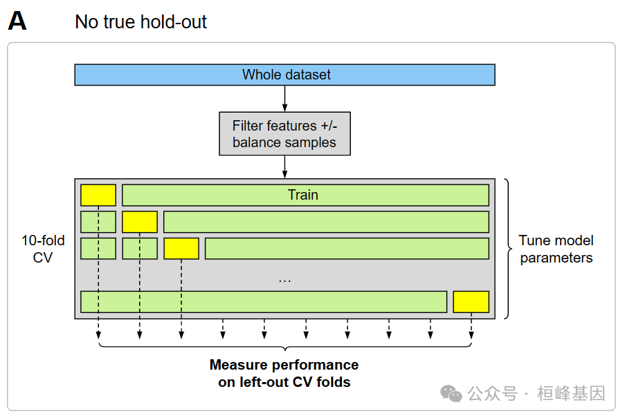
下面的图A和图B显示了两种常用但有偏差的方法,其中交叉验证用于拟合模型,但结果是对模型性能的有偏差估计。在方案A中,根本没有保留测试集,因此有两个偏差/数据泄漏的来源:首先,对整个数据集进行过滤,其次,使用遗漏的CV folds 来测量性能。已知遗漏的CV folds会导致对性能的偏差估计,因为调谐参数是从优化遗漏的CV folds 的结果中“学习”的。
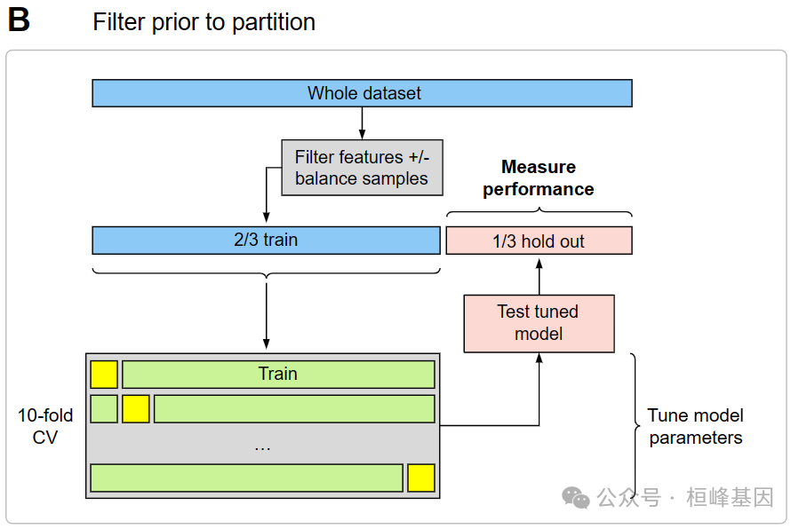
在方案B中,使用CV来调整参数,并使用保留集来衡量性能,但是当对整个数据集应用过滤时,会发生信息泄漏。不幸的是,这在许多研究中经常观察到,这些研究在整个数据集上应用微分表达式分析来选择预测因子,然后将其传递给机器学习算法。
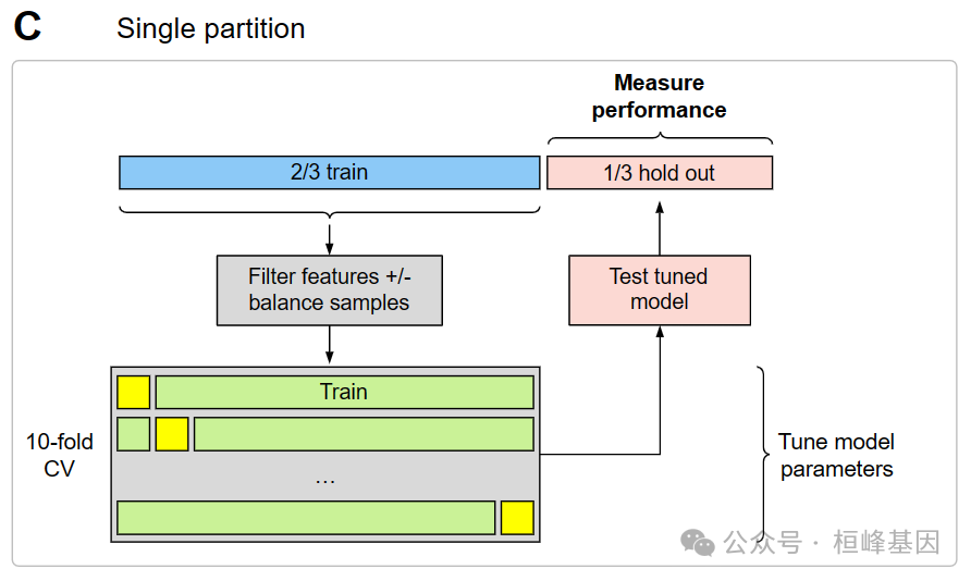
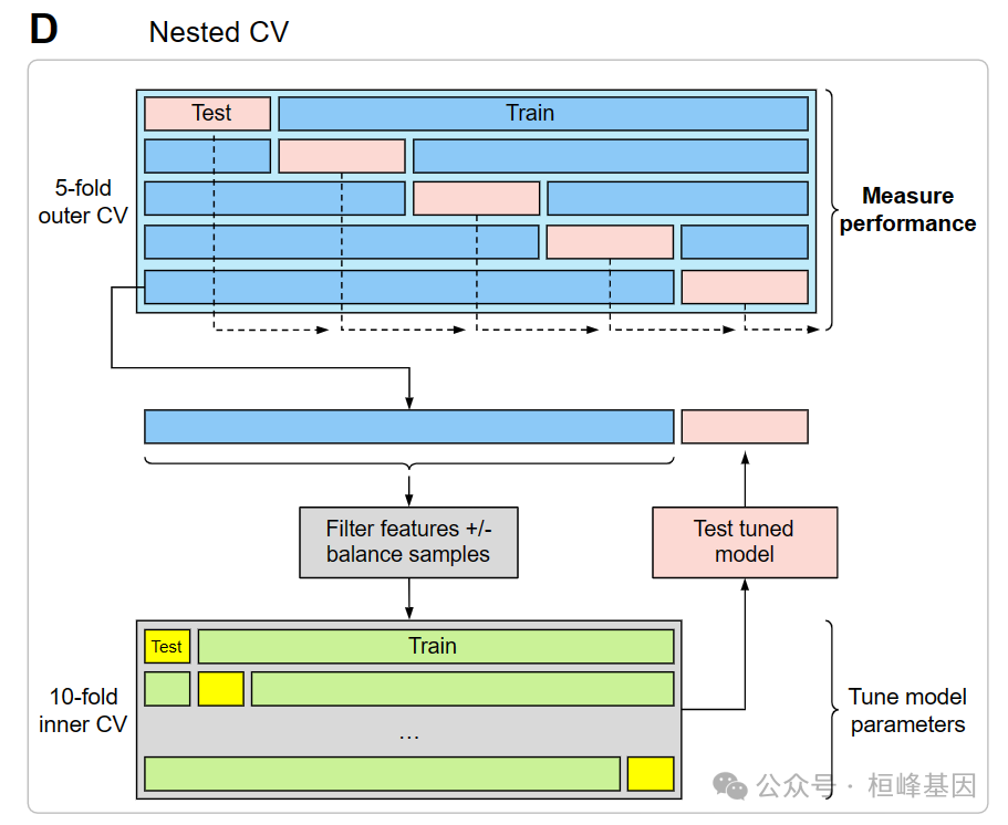
下面的图C和D显示了两种有效的方法,用于拟合具有CV的模型,用于调整参数以及模型性能的无偏估计。图C是一个传统的hold-out测试集,数据集被划分为2/3训练,1/3测试。值得注意的是,上述方案B之间的关键区别在于,过滤只在训练集上进行,而不是在整个数据集上进行。图D显示了完全嵌套交叉验证的方案。注意,过滤应用于每个外部CV训练folds。嵌套CV的主要优点是,与方案C相比,外部CV测试folds被整理,以提供更好的性能估计,因为总测试的数量更大。
虽然一些模型(如glmnet)允许稀疏性并内置变量选择,但当给定大量预测因子时,许多模型无法拟合,或者由于没有变量选择而过度拟合而表现不佳。此外,在医学中,预测建模的目标之一通常是开发诊断或生物标志物测试,因此减少预测因子的数量通常是实际需要。提供了几个用于特征选择的过滤函数(t-test, Wilcoxon test, anova, Pearson/Spearman相关性,随机森林变量重要性和CORElearn包中的ReliefF),并且可以嵌入到嵌套CV的外部循环中。下面的模拟示例演示了数据集固有的偏差。其中P>=n当对整个数据集应用预测器过滤时而不是去训练folds。
数据读取
数据来源《机器学习与R语言》书中,具体来自UCI机器学习仓库。地址:http://archive.ics.uci.edu/ml/machine-learning-databases/breast-cancer-wisconsin/ 下载wbdc.data和wbdc.names这两个数据集,数据经过整理,成为面板数据。查看数据结构,其中第一列为id列,无特征意义,需要删除。第二列diagnosis为响应变量,字符型,一般在R语言中分类任务都要求响应变量为因子类型,因此需要做数据类型转换。剩余的为预测变量,数值类型。查看数据维度,568个样本,32个特征(包括响应特征)。
BreastCancer <- read.csv("wisc_bc_data.csv", stringsAsFactors = FALSE)
str(BreastCancer)
## 'data.frame':	568 obs. of  32 variables:
##  $ id                     : int  842517 84300903 84348301 84358402 843786 844359 84458202 844981 84501001 845636 ...
##  $ diagnosis              : chr  "M" "M" "M" "M" ...
##  $ radius_mean            : num  20.6 19.7 11.4 20.3 12.4 ...
##  $ texture_mean           : num  17.8 21.2 20.4 14.3 15.7 ...
##  $ perimeter_mean         : num  132.9 130 77.6 135.1 82.6 ...
##  $ area_mean              : num  1326 1203 386 1297 477 ...
##  $ smoothness_mean        : num  0.0847 0.1096 0.1425 0.1003 0.1278 ...
##  $ compactne_mean         : num  0.0786 0.1599 0.2839 0.1328 0.17 ...
##  $ concavity_mean         : num  0.0869 0.1974 0.2414 0.198 0.1578 ...
##  $ concave_points_mean    : num  0.0702 0.1279 0.1052 0.1043 0.0809 ...
##  $ symmetry_mean          : num  0.181 0.207 0.26 0.181 0.209 ...
##  $ fractal_dimension_mean : num  0.0567 0.06 0.0974 0.0588 0.0761 ...
##  $ radius_se              : num  0.543 0.746 0.496 0.757 0.335 ...
##  $ texture_se             : num  0.734 0.787 1.156 0.781 0.89 ...
##  $ perimeter_se           : num  3.4 4.58 3.44 5.44 2.22 ...
##  $ area_se                : num  74.1 94 27.2 94.4 27.2 ...
##  $ smoothness_se          : num  0.00522 0.00615 0.00911 0.01149 0.00751 ...
##  $ compactne_se           : num  0.0131 0.0401 0.0746 0.0246 0.0335 ...
##  $ concavity_se           : num  0.0186 0.0383 0.0566 0.0569 0.0367 ...
##  $ concave_points_se      : num  0.0134 0.0206 0.0187 0.0188 0.0114 ...
##  $ symmetry_se            : num  0.0139 0.0225 0.0596 0.0176 0.0216 ...
##  $ fractal_dimension_se   : num  0.00353 0.00457 0.00921 0.00511 0.00508 ...
##  $ radius_worst           : num  25 23.6 14.9 22.5 15.5 ...
##  $ texture_worst          : num  23.4 25.5 26.5 16.7 23.8 ...
##  $ perimeter_worst        : num  158.8 152.5 98.9 152.2 103.4 ...
##  $ area_worst             : num  1956 1709 568 1575 742 ...
##  $ smoothness_worst       : num  0.124 0.144 0.21 0.137 0.179 ...
##  $ compactne_worst        : num  0.187 0.424 0.866 0.205 0.525 ...
##  $ concavity_worst        : num  0.242 0.45 0.687 0.4 0.535 ...
##  $ concave_points_worst   : num  0.186 0.243 0.258 0.163 0.174 ...
##  $ symmetry_worst         : num  0.275 0.361 0.664 0.236 0.399 ...
##  $ fractal_dimension_worst: num  0.089 0.0876 0.173 0.0768 0.1244 ...
dim(BreastCancer)
## [1] 568  32
table(BreastCancer$diagnosis)
##
##   B   M
## 357 211
data = na.omit(BreastCancer)
sum(is.na(data))  # 检测数据是否有缺失
## [1] 0
数据分割
虽然一些模型(如glmnet)允许稀疏性并内置变量选择,但当给定大量预测因子时,许多模型无法拟合,或者由于没有变量选择而过度拟合而表现不佳。此外,在医学中,预测建模的目标之一通常是开发诊断或生物标志物测试,因此减少预测因子的数量通常是实际需要。
## Example binary classification problem with P >> n
x <- as.matrix(data[, 3:31])  # predictors
y <- factor(ifelse(data$diagnosis == "M", 1, 0))  # binary response

## Partition data into 2/3 training set, 1/3 test set
trainSet <- caret::createDataPartition(y, p = 0.66, list = FALSE)
提供了几个用于特征选择的过滤函数(t-test, Wilcoxon test, anova, Pearson/Spearman correlation, random forest variable importance, and ReliefF from the CORElearn package),并且可以嵌入到嵌套CV的外部循环中。
## t-test filter using whole test set
library(nestedcv)
filt <- ttest_filter(y, x, nfilter = 100)
filx <- x[, filt]
实例操作
nestcv.glmnet()
下面的模拟示例演示了P >=N,当对整个数据集而不是训练CV应用预测器过滤时。
fit2 <- nestcv.glmnet(y, x, family = "binomial", alphaSet = 7:10/10, filterFUN = ttest_filter,
filter_options = list(nfilter = 100))
fit2
## Nested cross-validation with glmnet
## Filter: ttest_filter
##
## Final parameters:
## lambda alpha
## 0.001738 0.700000
##
## Final coefficients:
## (Intercept) fractal_dimension_se compactne_se
## -3.289e+01 -1.272e+02 -4.146e+01
## smoothness_worst concave_points_se concave_points_mean
## 3.826e+01 3.526e+01 2.606e+01
## concave_points_worst symmetry_worst compactne_mean
## 1.736e+01 1.006e+01 -8.497e+00
## radius_se concavity_mean concavity_worst
## 5.802e+00 5.526e+00 4.099e+00
## symmetry_mean radius_worst texture_worst
## -1.705e+00 3.371e-01 1.913e-01
## texture_mean perimeter_se perimeter_worst
## 9.584e-02 5.349e-02 3.822e-02
## area_se radius_mean area_worst
## 2.239e-02 3.171e-03 2.527e-03
## area_mean
## 4.273e-04
##
## Result:
## Reference
## Predicted 0 1
## 0 351 10
## 1 6 201
##
## AUC Accuracy Balanced accuracy
## 0.9950 0.9718 0.9679
metrics(fit2, extra = TRUE)
## AUC Accuracy Balanced accuracy PR.AUC
## 0.9949819 0.9718310 0.9679000 0.9885898
## Kappa F1 MCC nvar
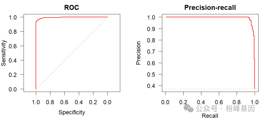
## 0.9394416 0.9617225 NA 21.0000000plot ROC and PR curves
虽然二元模型的ROC曲线对象是自动生成的,但对于嵌套的CV模型,可以使用使用ROCR包的方便函数prc()快速生成精度召回率曲线。
op <- par(mfrow = c(1, 2), mar = c(4, 4, 2, 2) + 0.1)
plot(fit2$roc, col = "red", main = "ROC", las = 1, ylim = c(0, 1), xlim = c(0, 1))
plot(fit2$prc, col = "red", main = "Precision-recall", ylim = c(0, 1), xlim = c(0,
    1))
Outer/Inner CV ROC
可以绘制出来自外部和内部CV的left-out folds 的ROC曲线。基于left-out outer folds 的AUC是对精度的无偏估计,而left-out inner folds由于对 inner fold 数据的模型超参数的优化而表现出偏差。
# Outer CV ROC
par(mfrow = c(1, 2))
plot(fit2$roc, main = "Outer fold ROC", font.main = 1, col = "blue")
legend("bottomright", legend = paste0("AUC = ", signif(pROC::auc(fit2$roc), 3)),
    bty = "n")

# Inner CV ROC
rtx.inroc <- innercv_roc(fit2)
plot(rtx.inroc, main = "Inner fold ROC", font.main = 1, col = "red")
legend("bottomright", legend = paste0("AUC = ", signif(pROC::auc(rtx.inroc), 3)),
    bty = "n")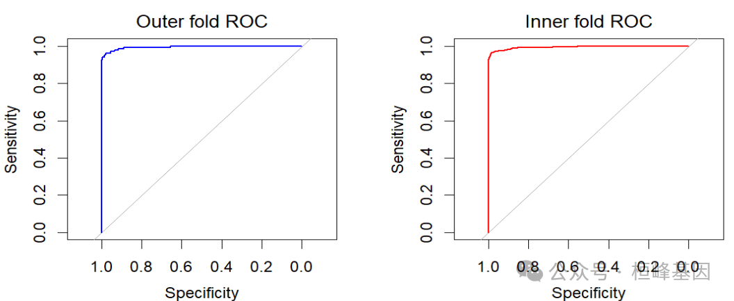
alpha的调整
可以绘制出每个外部倍数对alpha的调整。
par(mfrow = c(1, 3))
# Fold 1 line plot
plot(fit2$outer_result[[1]]$cvafit)

# Scatter plot
plot(fit2$outer_result[[1]]$cvafit, type = "p")

# Number of non-zero coefficients
plot(fit2$outer_result[[1]]$cvafit, xaxis = "nvar")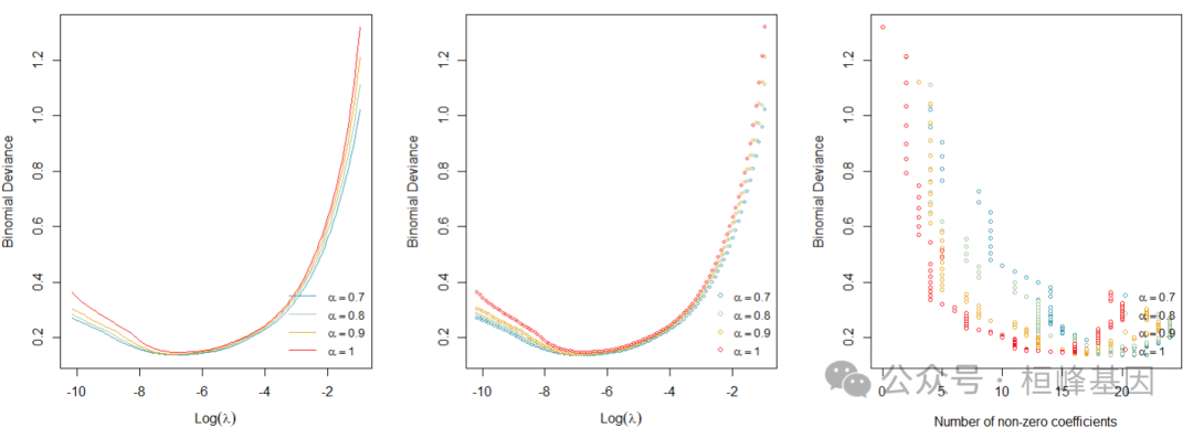
alpha和lambda分布
可以用glmnet绘制嵌套CV的输出,以显示偏差如何受到alpha和lambda的影响。
par(mfrow = c(1, 2))
plot_alphas(fit2)
plot_lambdas(fit2)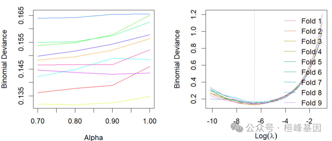
cv.glmnet()验证
## Train glmnet on training set only using filtered predictor matrix
library(glmnet)
fit <- cv.glmnet(filx[trainSet, ], y[trainSet], family = "binomial", type.measure = "auc")

## Predict response on test set
predy <- predict(fit, newx = filx[-trainSet, ], s = "lambda.min", type = "class")
predy <- as.vector(predy)
predyp <- predict(fit, newx = filx[-trainSet, ], s = "lambda.min", type = "response")
predyp <- as.vector(predyp)
output <- data.frame(testy = y[-trainSet], predy = predy, predyp = predyp)
## shows bias since univariate filtering was applied to whole dataset
predSummary(output)
##          Reference
## Predicted   0   1
##         0 119   3
##         1   2  68
##
##               AUC            Accuracy   Balanced accuracy
##            0.9853              0.9740              0.9706
testroc <- pROC::roc(output$testy, output$predyp, direction = "<", quiet = TRUE)
模型比较
最后,绘制ROC曲线来说明这些方法之间的差异。
inroc <- innercv_roc(fit2)
plot(fit2$roc)
lines(inroc, col = "blue")
lines(testroc, col = "red")
legend("bottomright", legend = c("Nested CV", "Left-out inner CV folds", "Test partition, non-nested filtering"),
    col = c("black", "blue", "red"), lty = 1, lwd = 2, bty = "n")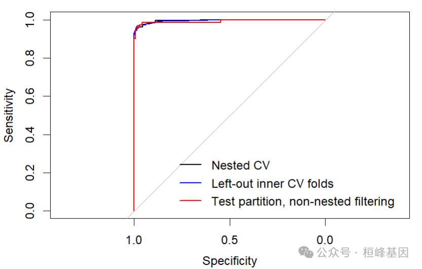
Reference
Lewis MJ, Spiliopoulou A, Goldmann K, Pitzalis C, McKeigue P, Barnes MR (2023). nestedcv: an R package for fast implementation of nested cross-validation with embedded feature selection designed for transcriptomics and high dimensional data. Bioinformatics Advances. https://doi.org/10.1093/bioadv/vbad048
基于机器学习构建临床预测模型
MachineLearning 2. 因子分析(Factor Analysis)
MachineLearning 3. 聚类分析(Cluster Analysis)
MachineLearning 4. 癌症诊断方法之 K-邻近算法(KNN)
MachineLearning 5. 癌症诊断和分子分型方法之支持向量机(SVM)
MachineLearning 6. 癌症诊断机器学习之分类树(Classification Trees)
MachineLearning 7. 癌症诊断机器学习之回归树(Regression Trees)
MachineLearning 8. 癌症诊断机器学习之随机森林(Random Forest)
MachineLearning 9. 癌症诊断机器学习之梯度提升算法(Gradient Boosting)
MachineLearning 10. 癌症诊断机器学习之神经网络(Neural network)
MachineLearning 11. 机器学习之随机森林生存分析(randomForestSRC)
MachineLearning 12. 机器学习之降维方法t-SNE及可视化(Rtsne)
MachineLearning 13. 机器学习之降维方法UMAP及可视化 (umap)
MachineLearning 14. 机器学习之集成分类器(AdaBoost)
MachineLearning 15. 机器学习之集成分类器(LogitBoost)
MachineLearning 16. 机器学习之梯度提升机(GBM)
MachineLearning 17. 机器学习之围绕中心点划分算法(PAM)
MachineLearning 18. 机器学习之贝叶斯分析类器(Naive Bayes)
MachineLearning 19. 机器学习之神经网络分类器(NNET)
MachineLearning 20. 机器学习之袋装分类回归树(Bagged CART)
MachineLearning 21. 机器学习之临床医学上的生存分析 (xgboost)
MachineLearning 22. 机器学习之有监督主成分分析筛选基因 (SuperPC)
MachineLearning 23. 机器学习之岭回归预测基因型和表型 (Ridge)
MachineLearning 24. 机器学习之似然增强Cox 比例风险模型筛选变量及预后估计 (CoxBoost)
MachineLearning 25. 机器学习之支持向量机应用于生存分析 (survivalsvm)
MachineLearning 26. 机器学习之弹性网络算法应用于生存分析 (Enet)
MachineLearning 27. 机器学习之逐步Cox回归筛选变量 (StepCox)
MachineLearning 28. 机器学习之偏最小二乘回归应用于生存分析 (plsRcox)
号外号外,桓峰基因单细胞生信分析免费培训课程即将开始快来报名吧!
桓峰基因,铸造成功的您!
未来桓峰基因公众号将不间断的推出单细胞系列生信分析教程,
敬请期待!!
桓峰基因官网正式上线,请大家多多关注,还有很多不足之处,大家多多指正!http://www.kyohogene.com/
桓峰基因和投必得合作,文章润色优惠85折,需要文章润色的老师可以直接到网站输入领取桓峰基因专属优惠券码:KYOHOGENE,然后上传,付款时选择桓峰基因优惠券即可享受85折优惠哦!https://www.topeditsci.com/


 991
991


 被折叠的 条评论
为什么被折叠?
被折叠的 条评论
为什么被折叠?
 到【灌水乐园】发言


