


简 介
可变剪接 (Alternative splicing) 是参与健康和疾病的重要机制。最近的工作强调了研究剪接模式的全基因组变化和随后的功能后果的重要性。目前的计算方法只支持这种基于基因的分析。因此,扩展了 IsoformSwitchAnalyzeR 库,以分析特定类型的选择性剪接的全基因组变化,并预测由此产生的异构体开关的功能后果。作为一个案例研究,分析了来自癌症基因组图谱的 RNA-seq 数据,发现了选择性剪接的系统性变化以及相关亚型开关的后果。
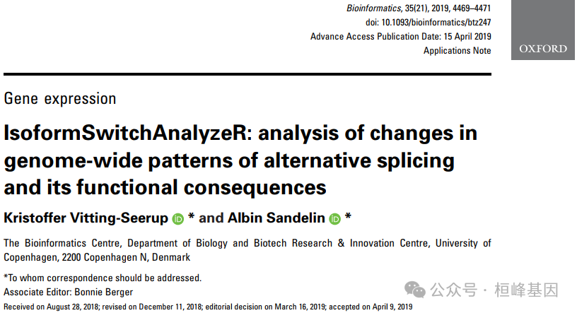
IsoformSwitchAnalyzeR 分析流程:
详细的工作流由以下步骤组成(如图下所示),就像前面一样,可以分为两个部分:
第1部分提取Isoform开关及其序列。
Importing Data Into R
Importing Data from Kallisto, Salmon, RSEM or StringTie
Importing Data from Cufflinks/Cuffdiff
Importing Data from Full-length Transcript Assemblers
Filtering
Identifying Isoform Switches
Analyzing Open Reading Frames
Extracting Nucleotide and Amino Acid Sequences
Advice for Running External Sequence Analysis Tools and Downloading Results
这对应于按顺序运行以下函数(顺便说一下,这正是isoformSwitchAnalysisPart1()函数所做的):
### Import data into R via one of:
myQantifications <- importIsoformExpression() # RSEM/Kallisto/Salmon/StringTie

### Create SwitchAnalyzeRlist
mySwitchList <- importRdata()         # OR
mySwitchList <- importCufflinksFiles()

### Filter
mySwitchList <- preFilter( mySwitchList )

### Test for isoform switches
mySwitchList <- isoformSwitchTestDEXSeq( mySwitchList )   # OR
mySwitchList <- isoformSwitchTestSatuRn( mySwitchList )

### If analysing (some) novel isoforms (else use CDS from ORF as explained in importRdata() )
mySwitchList <- addORFfromGTF( mySwitchList )
mySwitchList <- analyzeNovelIsoformORF( mySwitchList )

### Extract Sequences
mySwitchList <- extractSequence( mySwitchList )

### Summary
extractSwitchSummary(mySwitchList)
第2部分绘制所有同形开关及其注释。
Importing External Sequence Analysis
Predicting Alternative Splicing
Predicting Switch Consequences
Post Analysis of Isoform Switches with Consequences
Analysis of Individual Isoform Switching
Genome-Wide Analysis of Isoform Switching
这对应于按顺序运行以下函数(就像isoformSwitchAnalysisPart2()函数一样):
### Add annotation
mySwitchList <- analyzeCPAT( mySwitchList ) # OR
mySwitchList <- analyzeCPC2( mySwitchList )

mySwitchList <- analyzePFAM( mySwitchList )
mySwitchList <- analyzeSignalP( mySwitchList )

analyzeIUPred2A() # OR
analyzeNetSurfP2()

mySwitchList <- analyzeAlternativeSplicing( mySwitchList )

### Analyse consequences
mySwitchList <- analyzeSwitchConsequences( mySwitchList )

### Visual analysis
# Indiviudal switches
switchPlotTopSwitches( mySwitchList )

### Summary
extractSwitchSummary(mySwitchList, filterForConsequences = TRUE)
对于一个正常的工作流,接下来通常是对可变拼接和结果的全局分析:
# global consequence analysis
extractConsequenceSummary( mySwitchList )
extractConsequenceEnrichment( mySwitchList )
extractConsequenceGenomeWide( mySwitchList )

# global splicing analysis
extractSplicingSummary( mySwitchList )
extractSplicingEnrichment( mySwitchList )
extractSplicingGenomeWide( mySwitchList )
软件包安装
软件包安装非常简单,但是需要注意以下Rtools,R,BiocManager版本号,这种问题经常出现,更新匹配一直就没问题了。
if (!requireNamespace("devtools", quietly = TRUE)){
  install.packages("devtools")
}
if (!requireNamespace("pfamAnalyzeR", quietly = TRUE)){
  devtools::install_github("kvittingseerup/pfamAnalyzeR")
}

if (!requireNamespace("BiocManager", quietly = TRUE)){
  install.packages("BiocManager")
}
BiocManager::install(version='devel')
BiocManager::install("IsoformSwitchAnalyzeR")
数据准备
数据准备的过程比较复杂,这里需要准备5个文件,我们在做转录组分析时,可以获得注释文件 GFF或者GTF,count matrix, expression matrix,designMatrix 和 核酸序列 fasta。
第一步是将分析所需的所有数据导入 R,然后将它们连接为 switchAnalyzeRlist 对象。虽然 IsoformSwitchAnalyzeR 具有从Salmon/Kallisto/RSEM/StringTie/Cufflinks/IsoQuant (用于长读数据)等工具导入数据的不同功能,但 IsoformSwitchAnalyzeR 可以与任何产生同种异构体水平定量的工具的定量一起使用。为了说明将数据导入R的目的,让我们使用一些通过 Salmon 重新量化的袖扣数据,这些数据包含在 IsoformSwitchAnalyzeR 的分布中。
请注意:
如果使用Kallisto、RSEM或StringTie对数据进行量化,下面所示的鲑鱼数据方法是相同的。
如果您已经使用Salmon来量化Human/Mouse/Dropsophila Gencode/Ensembl 转录组的新版本,那么还有一种更简单的方法来导入数据 (使用taxmeta),如通过taxmeta从Salmon导入数据所述。
有关其他量化来源(包括StringTie和IsoQuant)。
import*() 等函数用于从不同数据源导入数据到 switchAnalyzeRlist 的函数,例如importsoformexpression()用于从Kallisto、Salmon StringTie或RSEM导入数据。
1. GFF/GTF文件格式及读入
gtf文件参考文件中必须还有的信息:
seqnames:染色体名称
ranges:起始-终止
type:外显子类型
transcript_id:转录本ID
gene_id:基因ID
gene_name:基因名称,一般就是symbol
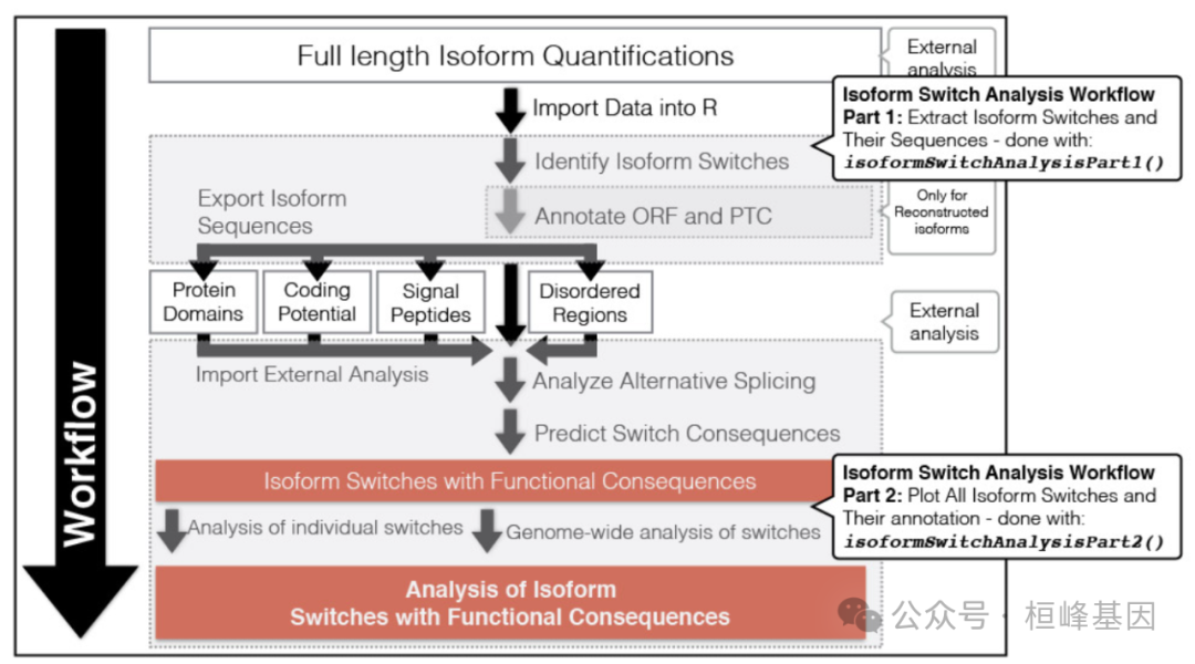
直接查看GTF文件,格式类似下面:
gtf的读入,有两种方式,一种 rtracklayer 包里面的 import(),另一种通过 IsoformSwitchAnalyzeR 包里面的 importGTF()
rtracklayer::import() 读入 GTF
library(rtracklayer)
isoformExonAnnoation = system.file("extdata/example.gtf.gz", package = "IsoformSwitchAnalyzeR")
test <- import(isoformExonAnnoation)
head(test)
## GRanges object with 6 ranges and 7 metadata columns:
##       seqnames      ranges strand |    source     type     score     phase
##          <Rle>   <IRanges>  <Rle> |  <factor> <factor> <numeric> <integer>
##   [1]     chr1 11874-12227      + | cufflinks     exon        NA      <NA>
##   [2]     chr1 11874-12227      + | cufflinks     exon        NA      <NA>
##   [3]     chr1 11874-12227      + | cufflinks     exon        NA      <NA>
##   [4]     chr1 12190-12227      + | cufflinks     CDS         NA      <NA>
##   [5]     chr1 12595-12721      + | cufflinks     CDS         NA      <NA>
##   [6]     chr1 12595-12721      + | cufflinks     exon        NA      <NA>
##        transcript_id     gene_id   gene_name
##          <character> <character> <character>
##   [1] TCONS_00000001 XLOC_000001        <NA>
##   [2] TCONS_00000002 XLOC_000001        <NA>
##   [3] TCONS_00000003 XLOC_000001        <NA>
##   [4] TCONS_00000002 XLOC_000001        <NA>
##   [5] TCONS_00000002 XLOC_000001        <NA>
##   [6] TCONS_00000002 XLOC_000001        <NA>
##   -------
##   seqinfo: 1 sequence from an unspecified genome; no seqlengths
IsoformSwitchAnalyzeR::importGTF() 读入 GTF
library(IsoformSwitchAnalyzeR)
gtfFile <- importGTF(pathToGTF = system.file("extdata/example.gtf.gz", package = "IsoformSwitchAnalyzeR"))
gtfFile
## This switchAnalyzeRlist list contains:
##  1092 isoforms from 375 genes
##  1 comparison from 2 conditions (in total 2 samples)
##
## Feature analyzed:
## [1] "ORFs"
这种读入方式可以方便我们查看GTF的具体情况,另外如果GTF不需要仔细查看确认也可以通过 importRdata() 函数直接读入到对象中:
### Create switchAnalyzeRlist
aSwitchList <- importRdata(
    isoformCountMatrix   = salmonQuant$counts,
    isoformRepExpression = salmonQuant$abundance,
    designMatrix         = myDesign,
    isoformExonAnnoation = system.file("extdata/example.gtf.gz"             , package="IsoformSwitchAnalyzeR"),
    isoformNtFasta       = system.file("extdata/example_isoform_nt.fasta.gz", package="IsoformSwitchAnalyzeR"),
    showProgress = FALSE
)
2. expression matrix 文件格式及读入
expression 矩阵的读入,有两种方式,一种 importIsoformExpression(),另一种通过 IsoformSwitchAnalyzeR 包里面的 importRdata()
1. importIsoformExpression() 读入表达矩阵
salmonQuant <- importIsoformExpression(parentDir = system.file("extdata/", package = "IsoformSwitchAnalyzeR"),
    addIsofomIdAsColumn = TRUE)

salmonQuant$abundance[1:5, ]
##       isoform_id Fibroblasts_0 Fibroblasts_1     hESC_0       hESC_1     iPS_0
## 1 TCONS_00000001      7.481356      7.969927       0.00 0.000000e+00  0.000000
## 2 TCONS_00000002      0.000000      0.000000       0.00 2.015807e+00  6.627746
## 3 TCONS_00000003      0.000000      6.116557       0.00 0.000000e+00  0.000000
## 4 TCONS_00000006  19052.485158      0.000000 6476850.47 2.709093e+06  0.000000
## 5 TCONS_00000007     21.758459     17.993108    1548.66 1.296613e+03 67.216637
##       iPS_1
## 1  5.320791
## 2  3.218813
## 3  0.000000
## 4  0.000000
## 5 75.426192
2. importRdata() 读入表达矩阵
这种读入方式可以方便我们查看表达矩阵的具体情况,另外如果表达矩阵不需要仔细查看确认也可以通过 importRdata() 函数直接读入到对象中:
### Create switchAnalyzeRlist
aSwitchList <- importRdata(
    isoformCountMatrix   = salmonQuant$counts,
    isoformRepExpression = salmonQuant$abundance,
    designMatrix         = myDesign,
    isoformExonAnnoation = system.file("extdata/example.gtf.gz"             , package="IsoformSwitchAnalyzeR"),
    isoformNtFasta       = system.file("extdata/example_isoform_nt.fasta.gz", package="IsoformSwitchAnalyzeR"),
    showProgress = FALSE
)
3. count matrix 文件格式及读入
count 矩阵的读入,有两种方式,一种 importIsoformExpression(),另一种通过 IsoformSwitchAnalyzeR 包里面的 importRdata()
这种读入方式可以方便我们查看 count 矩阵的具体情况,另外如果 count 矩阵不需要仔细查看确认也可以通过 importRdata() 函数直接读入到对象中:
salmonQuant$counts[1:5, ]
##       isoform_id Fibroblasts_0 Fibroblasts_1       hESC_0       hESC_1
## 1 TCONS_00000001      12.30707      14.02487      0.00000 0.000000e+00
## 2 TCONS_00000002       0.00000       0.00000      0.00000 1.116201e-01
## 3 TCONS_00000003       0.00000      10.76345      0.00000 0.000000e+00
## 4 TCONS_00000006   31341.93383       0.00000 163547.84518 1.500090e+05
## 5 TCONS_00000007      35.79335      31.66290     39.10543 7.179660e+01
##       iPS_0     iPS_1
## 1   0.00000  18.13313
## 2  21.10248  10.96964
## 3   0.00000   0.00000
## 4   0.00000   0.00000
## 5 214.01507 257.05074
### Create switchAnalyzeRlist
aSwitchList <- importRdata(
isoformCountMatrix = salmonQuant$counts,
isoformRepExpression = salmonQuant$abundance,
designMatrix = myDesign,
isoformExonAnnoation = system.file("extdata/example.gtf.gz" , package="IsoformSwitchAnalyzeR"),
isoformNtFasta = system.file("extdata/example_isoform_nt.fasta.gz", package="IsoformSwitchAnalyzeR"),
showProgress = FALSE
)4. designMatrix 写入
这个就是样本信息分组构造,很简单设计一个 data.frame() 即可:
myDesign <- data.frame(sampleID = colnames(salmonQuant$abundance)[-1], condition = gsub("_.*",
"", colnames(salmonQuant$abundance)[-1]))
myDesign
## sampleID condition
## 1 Fibroblasts_0 Fibroblasts
## 2 Fibroblasts_1 Fibroblasts
## 3 hESC_0 hESC
## 4 hESC_1 hESC
## 5 iPS_0 iPS
## 6 iPS_1 iPS5. 核酸序列读入
在构建对象是读入核酸序列fasta格式,设置 isoformNtFasta 参数:
### Create switchAnalyzeRlist
aSwitchList <- importRdata(
    isoformCountMatrix   = salmonQuant$counts,
    isoformRepExpression = salmonQuant$abundance,
    designMatrix         = myDesign,
    isoformExonAnnoation = system.file("extdata/example.gtf.gz"             , package="IsoformSwitchAnalyzeR"),
    isoformNtFasta       = system.file("extdata/example_isoform_nt.fasta.gz", package="IsoformSwitchAnalyzeR"),
    showProgress = FALSE
)以上数据都准备好了就可以构建 switchAnalyzeRlist 对象了。
### Create switchAnalyzeRlist
aSwitchList <- importRdata(isoformCountMatrix = salmonQuant$counts, isoformRepExpression = salmonQuant$abundance,
    designMatrix = myDesign, isoformExonAnnoation = system.file("extdata/example.gtf.gz",
        package = "IsoformSwitchAnalyzeR"), isoformNtFasta = system.file("extdata/example_isoform_nt.fasta.gz",
        package = "IsoformSwitchAnalyzeR"), showProgress = FALSE)
##            comparison estimated_genes_with_dtu
## 1 Fibroblasts vs hESC                  44 - 73
## 2  Fibroblasts vs iPS                  54 - 90
## 3         hESC vs iPS                  37 - 62
另外从 Cufflinks/Cuffdiff 导入数据是特别有趣的,因为 Cufflinks/Cuffdiff 是最广泛使用的重建异构体的工具之一(对于注释异构体的量化,我们推荐 Kallisto 或 Salmon 代替)。通过以下函数从 cufflinks data 创建 switchAnalyzeRlist:
library(cummeRbund)  # where the example data is stored

### Please note The way of importing file in this example with
### 'system.file('pathToFile', package='cummeRbund') is specialized way of
### accessing the example data in the IsoformSwitchAnalyzeR package and not
### something you need to do - just supply the string e.g.
### pathToGeneDEanalysis = '/myCuffdiffFiles/gene_exp.diff' to the argument.

testSwitchList <- importCufflinksFiles(pathToGTF = system.file("extdata/chr1_snippet.gtf",
    package = "cummeRbund"), pathToGeneDEanalysis = system.file("extdata/gene_exp.diff",
    package = "cummeRbund"), pathToIsoformDEanalysis = system.file("extdata/isoform_exp.diff",
    package = "cummeRbund"), pathToGeneFPKMtracking = system.file("extdata/genes.fpkm_tracking",
    package = "cummeRbund"), pathToIsoformFPKMtracking = system.file("extdata/isoforms.fpkm_tracking",
    package = "cummeRbund"), pathToIsoformReadGroupTracking = system.file("extdata/isoforms.read_group_tracking",
    package = "cummeRbund"), pathToSplicingAnalysis = system.file("extdata/splicing.diff",
    package = "cummeRbund"), pathToReadGroups = system.file("extdata/read_groups.info",
    package = "cummeRbund"), pathToRunInfo = system.file("extdata/run.info", package = "cummeRbund"),
    fixCufflinksAnnotationProblem = TRUE, quiet = TRUE)
testSwitchList
## This switchAnalyzeRlist list contains:
##  1203 isoforms from 468 genes
##  3 comparison from 3 conditions (in total 6 samples)
数据过滤
switchAnalyzeRlist 可能它包含了许多与异构体开关分析无关的基因/异构体。这样的例子可以是单同种异构体基因或非表达同种异构体。这些额外的基因/同种异构体将使下游分析花费比必要的时间。因此,在继续分析之前,实现了一个预过滤步骤来删除这些特征。重要的是,滤波可以增强下游分析的可靠性,使用 preFilter() 可以通过以下过滤从 switchAnalyzeRlist 的各个方面去除基因和同工型:
a). Multi-isoform genes
b). Gene expression
c). Isoform expression
d). Isoform Fraction (isoform usage)
e). Unwanted isoform classes
f). Unwanted gene biotypes
g). Genes without differential isoform usage
aSwitchList <- preFilter(switchAnalyzeRlist = aSwitchList, geneExpressionCutoff = 1,
    isoformExpressionCutoff = 0, removeSingleIsoformGenes = TRUE)


aSwitchList <- preFilter(switchAnalyzeRlist = aSwitchList, geneExpressionCutoff = 10,
    isoformExpressionCutoff = 3, removeSingleIsoformGenes = TRUE)
识别 isoform swtiches
由 于IsoformSwitchAnalyzeR 对 isoform swtiches 的识别至关重要,因此支持多种识别 isoform swtiches 的方法。目前,IsoformSwitchAnalyzeR 直接支持三种不同的方法:
1). DEXSeq:使用DEXSeq(最先进的)来测试差异异构体的使用。DEXSeq最初被设计用于测试差异外显子的使用,但最近被证明在差异异构体使用方面表现得非常好。可参考RNA 43. 基于转录组的外显子差异分析(DEXSeq)
2). satuRn :使用satuRn 包。参见RNA 44. 基于单细胞/bulk转录组的转录本差异分析(satuRn)。
3). Cufflinks/Cuffdiff:导入Cufflinks/Cuffdiff数据时,自动导入Cuffdiff执行的拼接分析。
但是,也可以使用其他工具的结果,这些工具可以在基因和/或异构体水平上测试差异异构体的使用。
1. 通过 DEXSeq 测试isoform Switches
测试差异异构体使用的两个主要挑战是控制错误发现率 (FDR) 和在具有混淆效应的实验设置中应用效应大小截止值。最近的研究,强调 DEXSeq 是一个很好的解决方案,因为它可以很好地控制 FDR。因此,在 IsoformSwitchAnalyzeR 中实现了一个基于 DEXSeq 的测试作为默认值。该测试进一步利用极限来产生校正混杂效应的效应量。
结果 isoformSwitchTestDEXSeq 是高度准确的,尽管随着分析的样本数量而严重扩展,但仍然比 DEXSeq 更快、更可靠——这就是为什么它目前是 IsoformSwitchAnalyzeR 中的默认(和推荐)测试。
### Test isoform swtiches
aSwitchList <- isoformSwitchTestDEXSeq(aSwitchList)
##
  |
  |                                                                      |   0%
  |
  |=======================                                               |  33%
  |
  |===============================================                       |  67%
  |
  |======================================================================| 100%

# extract summary of number of switching features
extractSwitchSummary(aSwitchList)
##            Comparison nrIsoforms nrSwitches nrGenes
## 1 Fibroblasts vs hESC          0          0       0
## 2  Fibroblasts vs iPS         72        102      44
## 3         hESC vs iPS        100         95      58
## 4            Combined        145        178      74
2. 通过 SatuRn 测试 isoform Switches
最近发布了satuRn软件包,提供了对差异异构体使用情况的可扩展和有效的分析。IsoformSwitchAnalyzeR 通过包装器 isoformSwitchTestSatuRn() 支持识别带有 satuRn 的isoform Switches,执行switchAnalyzeRlist中所有异构体的完整分析和比较。然后,将结果集成回 switchAnalyzeRlist 中,该列表像往常一样返回给用户。isoformSwitchTestSatuRn() 函数的使用如下:
mySwitchList <- isoformSwitchTestSatuRn(aSwitchList)
# extract summary of number of switching features
extractSwitchSummary(aSwitchList)
##            Comparison nrIsoforms nrSwitches nrGenes
## 1 Fibroblasts vs hESC          0          0       0
## 2  Fibroblasts vs iPS         72        102      44
## 3         hESC vs iPS        100         95      58
## 4            Combined        145        178      74
Reference
Vitting-Seerup K, Sandelin A. IsoformSwitchAnalyzeR: analysis of changes in genome-wide patterns of alternative splicing and its functional consequences. Bioinformatics. 2019 Nov 1;35(21):4469-4471.
桓峰基因,铸造成功的您!
未来桓峰基因公众号将不间断的推出生信分析系列教程,
敬请期待!!
桓峰基因官网正式上线,请大家多多关注,还有很多不足之处,大家多多指正!http://www.kyohogene.com/
桓峰基因和投必得合作,文章润色优惠85折,需要文章润色的老师可以直接到网站输入领取桓峰基因专属优惠券码:KYOHOGENE,然后上传,付款时选择桓峰基因优惠券即可享受85折优惠哦!https://www.topeditsci.com/


 被折叠的 条评论
为什么被折叠?
被折叠的 条评论
为什么被折叠?
 到【灌水乐园】发言


