OpenCV入门——Sobel, Canny, Laplace, Hough简介与代码实现

OpenCV入门——Sobel, Canny, Laplace, Hough简介与代码实现

Sobel Operator

Sobel operator is a very classic operator in edge extraction. First let’s consider how we can distinguish the edge in the whole picture. It’s clear that the color of the edge is totally different from it’s surrounding pixels. So if we can describe this situation in math, we can solve the problem. We know that if the change of function can be quantified using the first derivative. So considering the property of the edge the first derivative in the edge must be bigger than in’s surroundings. Now if we can calculate the first derivative of the image, it will be a big step to solve the problem and Sobel operator happens to realize it.

Usually one picture is stored with BGR formation which means there are three numbers representing the color in blue, green and red and the final color is the mixed result of these three colors. But it’s too complex when facing the math operating so we need to convert this kind of picture into gray picture. Gray picture is stored when every pixel is described using 8 bytes so the color is just from black to gray and finally to white. Under this situation, we can solve the math problems more easily. In my project, I use OpenCV in Ubuntu 16.04 to perform image processing. This step can be easily accomplished, and the results are below:

Now the problem is how to calculate the first derivative of the two-dimensional function. The equation is shown as

But the pixel in the picture is discrete so how to calculate? Well, the Sobel operator gives the answer. The operator uses two 3×3 kernels which are convolved with the original image to calculate approximations of the derivatives – one for horizontal changes, and one for vertical. If we define A as the source image, and G_x and G_y are two images which at each point contain the vertical and horizontal derivative approximations respectively, the computations are as follows:

Here G_x and G_y are convolution kernel. The total gradient norm can be calculated as:

The direction of gradient can be described as:

Thus all the parameters of first derivative are obtained. But we still don’t know where the edge is. In other words, we need a full procedure to detect the edge using Sobel operator, and that procedure is called Canny edge detector.

Canny edge detector

Although the Sobel operator is important to detect the edge, we need a full procedure to find out the edge and Canny algorithm gives us the answer.

1. Gaussian filter
   Almost every image has noise and it will influence the result of edge detecting a lot. So we need to use Gaussian filter to smooth the image first. The equation for a Gaussian filter kernel of size (2k+1)×(2k+1) is given by:

Similarly, we can use convolution process to perform Gaussian filter. For example, if σ is equal to 1.4, the convolution kernel is:

The result of Gaussian filter of gray image is shown as:

2. Finding the intensity gradient of the image
   Now the Sobel operator can do its job. We use Sobel operator to calculate the gradient and obtain the norm and direction of gradient function. It’s the fundamental of distinguishing edge. The theory has been talked before. We just use the Sobel convolution kernel to do the job.

3. Non-maximum suppression
   After step 2, we have the locations where the first derivative is big. However, it’s not clear enough for us to get the result because we want the edge to be as thin as possible. So we need the non-maximum suppression to preserve the maximum gradient point and abandon others. The procedure is firstly comparing the edge strength of the current pixel with the edge strength of the pixel in the positive and negative gradient directions. Then if the edge strength of the current pixel is the largest compared to the other pixels in the mask with the same direction (e.g., a pixel that is pointing in the y-direction will be compared to the pixel above and below it in the vertical axis), the value will be preserved. Otherwise, the value will be suppressed. For example, we have the pixel matrix as:
   
   Then it can be divided into four directions: 1 and 5 is one direction, 2 and 6 is one direction, 3 and 7, 4 and 8 are one direction respectively. If the gradient direction of center is along 3 and 7 direction, so we need to compare the gradient norm of center with 3 and 7, if the norm of center is bigger than both 3 and 7, then the center will be kept while 3 and 7 will be suppressed.

4. Double threshold
   After above steps, we have locations whose gradient norm is relatively biggest among surroundings. However, there are still lots of locations are kept because of noise. In order to account for these spurious responses, it is essential to filter out edge pixels with a weak gradient value and preserve edge pixels with a high gradient value. This is accomplished by selecting high and low threshold values. If an edge pixel’s gradient value is higher than the high threshold value, it is marked as a strong edge pixel. If an edge pixel’s gradient value is smaller than the high threshold value and larger than the low threshold value, it is marked as a weak edge pixel. If an edge pixel’s value is smaller than the low threshold value, it will be suppressed. The two threshold values are empirically determined and their definition will depend on the content of a given input image.

5. Edge tracking by hysteresis
   So far, the strong edge pixels should certainly be involved in the final edge image, as they are extracted from the true edges in the image. However, there will be some debate on the weak edge pixels, as these pixels can either be extracted from the true edge, or the noise/color variations. To achieve an accurate result, the weak edges caused by the latter reasons should be removed. Usually a weak edge pixel caused from true edges will be connected to a strong edge pixel while noise responses are unconnected. To track the edge connection, blob analysis is applied by looking at a weak edge pixel and its 8-connected neighborhood pixels. As long as there is one strong edge pixel that is involved in the blob, that weak edge point can be identified as one that should be preserved.

The result of canny algorithm is:

Hough transform

As we can see from the Canny algorithm result, there are lots of edges are lines which means lines are the basic geometric figure in edge extraction. So we should have some accurate way to determine the lines in the image. The Canny algorithm can only draw the edge but cannot decide if the geometric figure is a line. Now we need Hough transform.

A line can be written as:

So if we know the k and b this line is determined. In the other hand, we can also write a line as:

So if we consider x and y as the unknown parameters, b and k can be described as a line, too. Now let’s consider the relationship between the xy plane and bk plane. One point (x,y) in xy plane can determine one line in bk plane and the opposite is also true. As a pair of (b,k) determine a line in xy plane, if we choose different points in xy plane which are in the same line, the corresponding (b,k) should be same which means corresponding lines in bk plane of these points should pass through the same point (b,k) and this is our result.

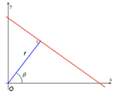
However, last equation has its limitations because the k can be infinite if the line is vertical to x axis. So we should use polar coordinates to solve the problem. The equation is shown as r=xcosθ+ysinθ and the image is:

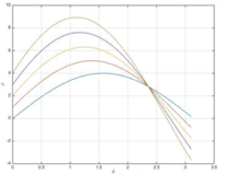
Similarly, one point (r,θ) in rθ plane represents a line in xy plane and one point (x,y) in xy plane represents a sine function curve in rθ plane. So if we choose different points in xy plane which are in the same line, the corresponding (r,θ) should be same which means corresponding lines in rθ plane of these points should pass through the same point (r,θ) and this is our result. Like the following picture, different points in xy plane is a sine curve, and they all pass through one point in rθ plane.

Now let's see how we can use this principle to determine a line. We simply divided the rθ plane into many small areas. Then we traverse all pixels in the image and draw the corresponding curves in rθ plane. Every area that the curve pass will increase the value. If the value is more than a threshold the corresponding rθ in that area can be seen as a line in the xy plane.

The result of Hough line detect is shown as below:

Laplace operator

As Sobel represents the first derivative of image intensity, the second derivative can also reflects some information. Laplace operation is:

When Laplace operator is 0 it also means the first derivative here is biggest. Similarly, we can also use convolutional operation to do the second derivative. The corresponding kernel is:

Now let’s see the result and compare it with Canny which use Sobel operator:

So it includes wider edge while Canny includes thinner edge. The noise of Laplace is much more than Canny because it doesn’t have Non-Maximum suppression. So Laplace operator is often used in sharpen to increase the contrast.

Code

#include <iostream>
#include <opencv2/opencv.hpp>
using namespace std;
using namespace cv;
int main() {
    Mat image_source,image_gray,image_gaussion,image_sobel,image_lap,image_bina,image_hough;
    image_source=imread("building.jpg",IMREAD_UNCHANGED);
    /*namedWindow("image_source",WINDOW_NORMAL);
    cvResizeWindow("image_source",1000,1000);
    imshow("image_source",image_source);*/
//import the source image

    cvtColor(image_source,image_gray,COLOR_BGR2GRAY);
    namedWindow("image_gray",WINDOW_NORMAL);
    cvResizeWindow("image_gray",1000,1000);
    imshow("image_gray",image_gray);
//transfer the source image to gray image

    GaussianBlur(image_gray,image_gaussion,Size(5,5),0,0);
    namedWindow("image_gaussion",WINDOW_NORMAL);
    cvResizeWindow("image_gaussion",1000,1000);
    imshow("image_gaussion",image_gaussion);
//Gaussian smoothing

    Canny(image_gaussion,image_sobel,500,20,5,true);
    namedWindow("image_sobel",WINDOW_NORMAL);
    cvResizeWindow("image_sobel",1000,1000);
    imshow("image_sobel",image_sobel);
//sobel

    Laplacian(image_gaussion,image_lap,CV_8U,5);
    convertScaleAbs(image_lap,image_lap);
    namedWindow("image_lap",WINDOW_NORMAL);
    cvResizeWindow("image_lap",1000,1000);
    imshow("image_lap",image_lap);
//laplacian

    threshold(image_lap,image_bina,0,255,THRESH_OTSU | THRESH_BINARY);
    namedWindow("image_bina",WINDOW_NORMAL);
    cvResizeWindow("image_bina",1000,1000);
    imshow("image_bina",image_bina);
//binaryzation

    vector<Vec2f> lines;
    HoughLines(image_sobel,lines,0.5,CV_PI/360,150);
    int numlines=0;
    for(size_t i=0;i<lines.size();i++){
        float rho=lines[i][0],theta=lines[i][1];
        Point p1,p2;
        double a=cos(theta),b=sin(theta);
        double x0=rho*a,y0=rho*b;
        p1.x=cvRound(x0+1000*(-b));
        p1.y=cvRound(y0+1000*a);
        p2.x=cvRound(x0-1000*(-b));
        p2.y=cvRound(y0-1000*a);
        line(image_source,p1,p2,Scalar(55,100,95),1,CV_AA);
        numlines++;
    }
    cout<<numlines<<endl;
    namedWindow("image_hough",WINDOW_NORMAL);
    cvResizeWindow("image_hough",1000,1000);
    imshow("image_hough",image_source);
//Hough line
    waitKey();
    return 0;
}