四旋翼轨迹规划最优控制

本篇介绍了给定四旋翼起始状态，包括位置、速度、加速度、加加速度jerk、加加加速度jounce，并且给定末端状态，根据最优控制理论，规划从起点到终点途中各状态与时间的变化关系。

Optimum Control of Quadcopter

There are numbers of trajectories that a quadcopter can choose given the initial state and final state. So we need to choose the relatively best one to minimize the parameters we care about. That’s not easy but we still have a ripe theory called optimum control to realize our purpose.

A. Formulating the Dynamics in Jerk

For this linear acceleration equation:

Where f is the amplitude of acceleration, e_3 f is the acceleration vector in the body frame and Re_3 f is the same acceleration vector but written in the inertial frame. So the amplitude of Re_3 f is as same as f and thus the amplitude of f can be calculated in Euclidean norm:

Given a thrice differentiable motion x(t), the jerk which is derivation of acceleration can be written as j=x ⃛=(x ⃛_1,x ⃛_2,x ⃛_3 ). So if we take the first derivative of x ̈=Re_3 f+g yields:

Remember R ̇=R([w×] ) ̅ so we can get:

Then as we don’t know the derivation of f yet we take the derivation of ‖f‖=‖x ̈-g‖ and the result is:

Here is the process:
As we know the definition of Euclidean norm so f is specifically as:

So the first derivation of the last equation is:

If we transfer the last equation into the form of matrix we can get:

From x ̈=Re_3 f+g we can easily get:

After substitution of (x ̈-g)^T we can get the final result:

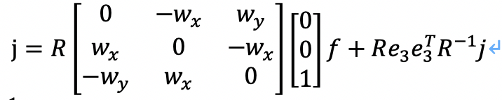
Now we can substitute f ̇ and ([w×] ) ̅ in j=R([w×] ) ̅e_3 f+Re_3 f ̇ we can obtain:

Note that w_1 and w_2 here is the angular velocity in the body frame.
Here is the process:
After substitution we can get:

Then we pre-multiply R^(-1) in both sides of the equation and we get:

Now it’s not difficult to obtain the final equation:

If we consider the air resistance, the equation is complex:

So till now we get the formulation of dynamics in jerk which is very important in the following analysis.

B. Cost Function

In order to obtain the optimum trajectory and input we need a cost function to judge the whole state of flying. It’s obvious that the goal is to generate a trajectory which guides the quadcopter from in initial state to a final state in a final time T while minimizing the cost function. In this place we can define the cost function as this:

This cost function has an interpretation as an upper bound on the average of a product of the inputs to the quadcopter system which means:

Where R^(-1) is a rotation matrix so it won’t change the amplitude of j and [■(1&0&0@0&1&0@0&0&0)] erase the third element of j so it must have:

So that:

This cost function is also computationally convenient and it’s a closed-form solution.

C. Axis Decoupling and Trajectory Generation

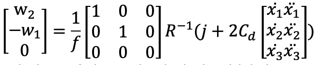
The nonlinear trajectory generation problem is simplified by decoupling the dynamics into three orthogonal inertial axes and treating each axis as a triple integrator with jerk used as control input. Of course jerk is not the true input while the true input is f and w but they can be recovered from ‖f‖=‖x ̈-g‖ and [■(w_2@-w_1@0)]=1/f [■(1&0&0@0&1&0@0&0&0)] R^(-1) j . Now let’s generate the trajectory using optimum control theory for each axis.
The first step is to decouple the cost function J_∑▒ in to per-axis cost J_k by expanding the integrand the cost function:

Where

For each axis k, the state s_k=(p_k,v_k,a_k ) is introduced, consisting of the scalars position, velocity, and acceleration. So that:

Notice that f_s is a function relates the state s_k and input j_k with derivation of state which is s ̇_k, this function will be used in optimum control theory. For the sake of readability, the axis subscript k will be discarded for this section where only a single axis is considered.

An optimal control is a set of differential equations describing the paths of the control variables that minimize the cost function. As we have a cost function and state space equation for our problem we can now using Pontryagin’s principle and Hamilton–Jacobi–Bellman equation to solve the optimum control. Let’s introduce a abstract framework of optimum control. The cost function is written as:

Where t_0 and t_f is the initial time and final time respectively, Φ is a function which means cost function is related to the initial state and final state of the problem. For our problem here, we have no Φ because we don’t use the initial and final state to judge our trajectory. It’s obvious in our problem, L[x(t),u(t),t] is equal to 1/T j_k (t)^2.

In the abstract framework the state equation is in the following form:

Which in our problem a is equal to f_s, x(t) is equal to s_k and u(t) is equal to j_k (t). Sometimes there are boundary conditions in the abstract framework which is:

which means there are constrains of the state in the inertial or final state. In our problem it’s not decided for now because it can be determined in different situations. For example, we want the quadcopter to be in a specified position and velocity in the end state so we can define a corresponding boundary conditions ψ to constrain the final state. It will be discussed later.
Now we have the cost function, state equation and boundary conditions, so how do we calculate the optimal control? Here is the answer. We can introduce the costate λ(t) and define the Hamiltonian function H(x,u,λ,t)=L[x(t),u(t),t]+〖λ〗^T (t)a[x(t),u(t),t], and following equations must be satisfied:

Where λ(t_f )=0 should be satisfied when there is no constrain in corresponding state and the last equation should be satisfied when t_f is free. Notice that superscript * means the optimum parameter which we are supposed to obtain. Now let’s begin dealing with our own problem by establishing Hamiltonian function first:

Why λ ̇=-∂H/∂x is equal to λ ̇=-∇_s H(s,j,λ)? As ∂H/∂x is an operation in functional analysis we only give the result of this:

We also have:

Where I,j,k is the unit direction vector. So -∇_s H(s,j,λ) is also equal to –(∂H/∂p,∂H/∂v,∂H/∂a)
The costate differential λ ̇=(0,-λ_1,-λ_2 ) is easily solved and the result is:

where α,β,γ are all constants and will be solved later.
The optimal input trajectory is solved according to H(x^*,u,t)=minH(x^,u,t) ,u∈Ω as:

As we find that H(s,j,λ)=1/T j^2+λ_1 v+λ_2 a+λ_3 j is a quadratic function with respect to j so the minimum can be reached when j equals to the symmetrical axis which is -λ_3/(2 1/T), so we have:

So we get j^* which is the optimal input which can minimize the cost function. Next step is to obtain the corresponding s^* which is the optimal state when quadcopter fly. It can be done through the integration of j. Let’s see the process. The state equation is:

So a ̇_k=j_k. Then through the integration of j we can get:

Where a_0 is acceleration at the inertial time. Similarly we can get the v_k and p_k through the double integration and triple integration of j and the result is:

Where the inertial state is s_0=(p_0,v_0,a_0 )

The remaining unknown α,β,γ can be solved depending on boundary conditions. It can be divided into two classes.

1. Fully Defined End Translational State: This class means we define all the state in the final state which is (p_f,v_f,a_f ). So s^* (T) must equal to (p_f,v_f,a_f ) and we have:
   
   Where
   
   So we can get unknown coefficients:
   
   Till now the optimal control of this class is solved. As we know the (α,β,γ) we can obtain the (p,v,a,j) in every second of flying.
2. Partially Defined End Translational State: This class means we define part of state in the final state. For example, we define that at the final time only position and velocity should satisfy (p_(f),v_f) while acceleration can be free. So under this situation s^* (T) is not equal to (p_f,v_f,a_f ) anymore because a_f is not defined. But the first two lines which are s^* (T)=(p_f,v_f) are still correct because p_f and v_f are still defined. We are supposed to use λ_3 (t_f )=0 which is also the criterion of optimum control so that we have three equations to calculate three unknown coefficients (α,β,γ). So we have:
   
   The first two equations are not changed as s^* (T)=(p_f,v_f) and the third equation is λ_3 (t_f )=0 which is -αt^2-2βt-2γ=0. Then write them in the form of matrix we can get the above result. So the unknown coefficient can be solved:
   
   As the third column of right side is all zero when calculating so we can also write in this form:
   
   Of course we can define position and acceleration at the end time. So there are all 7 different combinations including the two we have discussed. The result is listed as following:
   Fixed Position, Velocity, and Acceleration
   
   Fixed Position and Velocity
   
   Fixed Position and Acceleration
   
   Fixed Velocity and Acceleration
   
   Fixed Position
   
   Fixed Velocity
   
   Fixed Acceleration
   
   After we get (α,β,γ) we can calculate cost function in a more easy way. As J_k=1/T ∫_0^T▒〖j_k (t)^2 dt〗 and j^* (t)=1/2 αt^2+βt+γ we can solve cost function into this:
   
   Note that this holds for all combinations of end translational variables.

D. Formulating the Dynamics in Jounce

We have already obtain all results when the input is jerk. However, it has some problems. We can determine the angular velocity using this equation without considering the resistance:

So using the optimal control theory if the jerk is input, it is

At the initial time which means t=0 so j=γ. And we can assure γ cannot be zero.

Because if we want γ be zero, the third row of this equation must be satisfied in all three axis. But as there is only T one variable value and there are three equations so it can’t be satisfied.
Now let’s consider the real case. If we want the quadcopter fly from the ground, at the beginning time the angular velocity must be zero. But if jerk is not zero at the beginning, the angular velocity can’t be zero so it’s not practical. Therefore, we must control the j to be zero at the initial time so we need to control the derivative of jerk which is jounce h to accomplish our purpose. Similarly, we can build up the Hamiltonian function:

Cost function:

So we can obtain:

So we can get the optimal jounce:

The state is:

So the coefficients can be obtained:

Input Feasibility

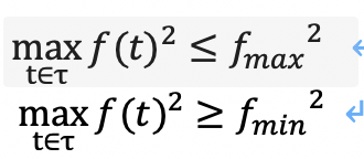
In the above trajectory designing we don’t consider the input feasibility. On the one hand, the thrust f should satisfy:

Where f_min and f_max are decided by the parameter of propellers. On the other hand, the magnitude of the angular velocity should be constrained:

Where w_max can be determined by the saturation limits of the rate gyroscope or motion limits of cameras mounted on the vehicle. Now let’s consider thrust first.

1. Thrust: We consider the time interval of our motion is τ=[τ_1,τ_2 ]⊆[0,T] first and later I will talk about how to guarantee all the time in [0,T] are feasible for input. It is obvious that we the thrust should satisfy:
   
   But it’s a little bit complex to consider all three axis one time so we decompose the thrust to each coordinate axis. We have:
   
   By taking the per-axis extrema of the last equation, we have:
   
   The first equation is obvious because the maximum (x ̈_k-g_k )^2 is definitively smaller than it’s corresponding magnitude in three axis and the latter is smaller than the right side of inequation. The second and third inequation are correct because maximum (x ̈_k-g_k )^2 in three different axis can be taken at different times and all of them are larger than projection on each axis of max┬(t∈τ)⁡〖f(t)^2 〗. So we have following three criterions:

If there is one axis that meets max┬(t∈τ)⁡〖(x ̈_k-g_k )^{2≥max┬(t∈τ)⁡〖f(t)}2 〗 〗, it’s definitely infeasible.

If the sum of maximum of all of three which is smaller than the upper-bound, which means max┬(t∈τ)⁡〖f(t)^2 ≥〗 ∑_(k=1)^3▒〖max┬(t∈τ) (x ̈_k-g_k )〗^2 , it’s definitely feasible.

If the sum of minimum of all of three which is bigger than the lower-bound, which means min┬(t∈τ)⁡〖f(t)^2 ≤〗 ∑_(k=1)^3▒〖min┬(t∈τ) (x ̈_k-g_k )〗^2 , it’s definitely feasible.

As we have mentioned before, if we know all the three states in both beginning time and final time, x ̈_k-g_k is a third-order polynomial in time, meaning the maximum and minimum (denoted ¯(x ̈_k ) and ▁(x ̈ )_k respectively) can be found from solving for the root of j=0 and at the boundaries of τ. So the extrema of (x ̈_k-g_k )^2 then follow as:

2) Body Rates: As we have mentioned before f^2 ‖w‖^2≤‖j‖2 so we have:

So if ¯w^2≤w_max2 it’s definitely feasible.
3) Recursive Implementation: What we have done above is in τ=[τ_1,τ_2 ] but the final purpose is to verify the feasibility of [0,T]. The process we are going to do is similar to dichotomy. First we divide τ=[τ_1,τ_2 ] to two components like this:

If both τ_before and τ_after are both feasible, the result is definitely feasible. If one of them is infeasible, the whole time is infeasible. If there is no infeasible time interval and there is indeterminate time interval, we continue repeat the above process for indeterminate time interval. Finally if the time interval is smaller than user-defined minimum Δτ, the algorithm terminates with the result indeterminable.

Example of Optimal Control

In order to testify all the equations we have derived are correct, I have made an easy example and plot the image in MATLAB. The initial states are quite simple that all the states including position, velocity and acceleration in all directions are zero. The final acceleration of Z axis is -2g which means the quadcopter is upside down at the end, and the final position of X axis is 10m.

So according to the final and initial state we can quickly obtain the coefficients (α,β,γ) and state functions with regard to time. Let’s see the result graphic.

First three graphics can be easily obtained because the state including acceleration, velocity, position and jerk are already known according to optimal control. However, angular velocity is a little bit difficult to calculate as it is concerned to the rotation matrix. Now I will introduce the way to calculate angular velocity.

We have the equation:

As f and j are both known so the key to calculate w is to calculate R^(-1). But as we have mentioned before, different rotation sequence has different R. So we choose two sequences which are XYZ and ZYX. But no matter what kind of sequence we choose, our model does not come down to the ϕ and ψ in theory. So we can calculate without rotation matrix just consider θ. The equations are shown as below:

It’s very important that when calculate the inverse trigonometric we have to notice arcsin cannot be less than -π/2 which is not true in our model. As at the end moment, the acceleration is -2g which means the angular is -π so when acceleration in Z axis is smaller than zero, we should process the final result properly. So the equations are these:

Finally when we get the result θ function with respect to time. ϕ and ψ keep zero as I mentioned. So 〖R^(-1)=R〗_y(-1)=[■(cosθ&0&-sinθ@0&1&0@sinθ&0&cosθ)]. Then we can obtain w_1 and w_2 respectively.

Now let’s consider ZYX sequence. The rotation matrix of ZYX is:

Then substitute this into:

We can get:

As we already know all parameters except ϕ,θ,φ we can calculate this equation in MATLAB. But this is a trigonometric function equation of degree three so it has different result at the same time and cannot be calculated very precisely. The result graphic of w and error are:

Error means we substitute the result calculated from the MATLAB into the original equation to see if the original equation is zero. From the graphic we can see there are lots of points where the result are not precise. So this ZYX sequence is not proper.

Now let’s see XYZ sequence. The rotation matrix is:

Similarly we can get:

This equation is much easier than ZYX one and it’s not related to ψ so it’s a equation of degree two with easier form. Why is this equation not related to ψ? It’s reasonable because ψ will not influence the linear motion at all.

The result is very close to the ideal one when we ignore ϕ and ψ as zero. The graphic of w is almost same so I only put the error graphic:

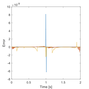
From the Y axis we can see the error is not zero but it can be ignored so this result is more reliable. Hence we use XYZ sequence in our following research.