SLAM中线特征的参数化和求导过程（从前端提取，到后端优化）

背景

线特征的提出，是在这样一个大背景下，基于点特征的视觉slam系统，平时没问题，但遇到了缺乏纹理的甚至是完全没有纹理的low-texured场景。可能会失效。 线特征的出现就是更加充分的利用了空间中领的这些几何信息，那么自然视觉slam系统也就会更加的鲁棒。
点特征我们很熟悉，前端提取，后面把它的空间三维坐标（也恰好是三个自由度）输入到后端优化器中尽心优化。因为恰好是三自由度，三个坐标，所以没有多余的约束，可以使用无约束条件的非线性优化。利用的库就是ceres，g2o和GTSAM那些。
现在，线特征如果要引入基于优化的视觉slam系统，一定也需要面对这样的问题。点特征在后端使用了“重投影误差”，也即时3D的点反投影回到像素平面和像素平面直接提取出的观测值2D点坐标进行一个做差处理。需要思考，对于线特征，我们要弄一个怎样的差，也就是常说的residual出来，并且求出residual对于待优化变量，比如相机的位姿和线特征的坐标，的雅可比矩阵，有了这些要素，直接使用开源优化库框框一顿计算就好了。

下面我们就来详细介绍一下空间直线的两种参数化方法：Plücker参数化方法，直线正交表示方法。为什么需要两种参数化方法呢？因为空间中的直线有4个自由度，而Plücker参数化方法需要使用6个参数表示直线，这样就会导致过参数化，过参数化在优化的时候就需要采用带约束的优化，不太方便。于是引入了可以用4个参数更新直线的正交表示来方便优化。这两种参数化方法可以很方便的相互转换，所以我们可以在SLAM系统中同时使用这两种参数化形式，在初始化和进行空间变换的时候使用Plücker坐标，在优化的时候使用正交表示。下面我们就来详细了解这两种参数化方法和优化的雅克比求导。

数学模型

1、Plücker参数化方法

在3D空间中，直线 $\mathcal{L}$ 的Plücker坐标表示为$\mathcal{L}={\left({\mathbf{n}}^{\top },{\mathbf{d}}^{\top }\right)}^{\top }\in R^6$ ，其中 $\mathbf{d}\in {\mathbf{R}}^3$是直线的方向向量， $\mathbf{n}\in {\mathbf{R}}^3$ 是由直线和光心构成的平面 的法向量。Plücker坐标是过参数化的，overparameterized（6个坐标值，却只有4个自由度DoF），比如 和 之间存在约束关系 $\left({\mathbf{n}}^{\top }\mathbf{d}=0\right)$。于是Plücker坐标不能直接使用无约束的优化。不过这种使用法向量和方向向量的表现形式在初始化直线和进行空间变换的时候很方便。所以在SLAM系统中我们可以使用Plücker坐标来初始化和变换，具体的初始化和变换方法如下：

当给定从世界坐标系 $w$ 到相机 $c$ 的变换矩阵$T_{cw}=\left[\begin{array}{cc}{R}_{cw}& p_{cw}\\ 0& 1\end{array}\right]$,可以通过下面的形式将世界坐标系和相机坐标系下的Plücker线坐标进行变换：
${\mathcal{L}}^c=\left[\begin{array}{l}{\mathbf{n}}^c\\ {\mathbf{d}}^c\end{array}\right]={\mathcal{T}}_{cw}{\mathcal{L}}_w=\left[\begin{array}{cc}{\mathbf{R}}_{cw}& {\left[{\mathbf{p}}_{cw}\right]}_{\times }{\mathbf{R}}_{cw}\\ 0& {\mathbf{R}}_{cw}\end{array}\right]{\mathcal{L}}^w$

上式中 $[\cdot {]}_x$ 表示的是三维向量的反对称矩阵，${\mathcal{T}}_{cw}$ 表示的是从世界坐标 $w$到相机坐标$c$ 的Plücker线坐标的变换矩阵, 跟三维点的坐标变换矩阵比较像但是略有不同。
$[a{]}_{\times }=\left[\begin{array}{l}{a}_1\\ a_2\\ a_3\end{array}\right]=\left[\begin{array}{ccc}0& -a_3& a_2\\ a_3& 0& -a_1\\ -a_2& a_1& 0\end{array}\right]$

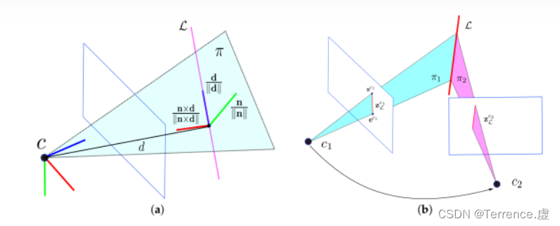
当我们从不同的两帧相机观测到一个新的线路标的时候，Plücker坐标初始化方式也很简单。如图1b中所示，直线 $\mathcal{L}$ 在两帧图像$c_1$ 和$c_2$ 中表示为两个线段${\mathbf{z}}_{\mathcal{L}}^{c_1}$ 和 ${\mathbf{z}}_{\mathcal{L}}^{c_2}$ 。线段 在归一化平面可以被两个端点表示， ${\mathbf{s}}^{c_1}={\left[\begin{array}{lll}{u}_{\mathrm{s}}& v_{\mathrm{s}}& 1\end{array}\right]}^T$ 和 ${\mathbf{e}}^{c_1}={\left[\begin{array}{lll}{u}_{\mathrm{e}}& v_{\mathrm{e}}& 1\end{array}\right]}^T$ 。再加上坐标原点 $\mathbf{C}=\left[\begin{array}{lll}{x}_0& y_0& z_0\end{array}\right]$ ，这三个点可以确定一个平面: $\pi =\left[\begin{array}{llll}{\pi }_x& {\pi }_y& {\pi }_z& {\pi }_w\end{array}\right]$.

${\pi }_X\left(x-x_0\right)+{\pi }_y\left(y-y_0\right)+{\pi }_z\left(z-z_0\right)=0$

其中： $\left[\begin{array}{l}{\pi }_x\\ {\pi }_y\\ {\pi }_z\end{array}\right]={\left[{\mathbf{s}}^{c1}\right]}_{\times }{\mathbf{e}}^{c_1},{\pi }_w={\pi }_x{x}_0+{\pi }_y{y}_0+{\pi }_z{z}_0$
然后从对偶矩阵中可以提取出Plücker坐标， $\mathcal{L}={\left({\mathbf{n}}^T,{\mathbf{d}}^T\right)}^T$ ，法向量和方向向量都不要求一定要是单位向量。

2、正交表示法

3D空间下的直线只有4个自由度，使用Plücker坐标的话，是过参数化的表示形式，在优化过程是有约束的不方便，所以引入一种四个参数的表达方式这样就没有多余的约束了，此处就是一种正交表示： $(\mathbf{U},\mathbf{W})\in SO(3)\times SO(2)$ 。 这两种形式之间的转换是很方便的。

首先我们需要知道了直线的Plücker坐 $\mathcal{L}={\left({\mathbf{n}}^{\top },{\mathbf{d}}^{\top }\right)}^{\top }$ ，然后对 进行QR分解，得到：

$\left[\begin{array}{ll}\mathbf{n}& \mathbf{d}\end{array}\right]=\left[\begin{array}{lll}\frac{\mathbf{n}}{\Vert \mathbf{n}\Vert }& \frac{\mathbf{d}}{\Vert \mathbf{d}\Vert }& \frac{\mathbf{n}\times \mathbf{d}}{\Vert \mathbf{n}\times \mathbf{d}\Vert }\end{array}\right]\left[\begin{array}{cc}\Vert \mathbf{n}\Vert & 0\\ 0& \Vert \mathbf{d}\Vert \\ 0& 0\end{array}\right]$
分解得到的第一项是正交矩阵 $\mathbf{U}$，是一个旋转矩阵。所表示的是相机坐标系到直线坐标系的旋转。其中直线坐标系的定义如下：用直线的方向向量以及直线和光心组成平面的法向量作为坐标的两个轴，再用他们叉乘得到的向量作为第三个轴，所以

$\begin{array}{rl}\mathbf{U}& ={\mathbf{R}}_x\left({\theta }_1\right){\mathbf{R}}_y\left({\theta }_2\right){\mathbf{R}}_z\left({\theta }_3\right)=\left[\begin{array}{lll}{\mathbf{u}}_1& {\mathbf{u}}_2& {\mathbf{u}}_3\end{array}\right]\\ & =\left[\begin{array}{lll}\frac{\mathbf{n}}{\Vert \mathbf{n}\Vert }& \frac{\mathbf{d}}{\Vert \mathbf{d}\Vert }& \frac{\mathbf{n}\times \mathbf{d}}{\Vert \mathbf{n}\times \mathbf{d}\Vert }\end{array}\right]\end{array}$

对于后面矩阵的两个元素 $\Vert \mathbf{n}\Vert ,\Vert \mathbf{d}\Vert$ 实际上只有一个自由度，把它们归一化以后，就能用一个$SO2$来更新它
$\begin{array}{rl}\mathbf{W}& =\left[\begin{array}{cc}\cos (\varphi )& -\sin (\varphi )\\ \sin (\varphi )& \cos (\varphi )\end{array}\right]=\left[\begin{array}{cc}{w}_1& -w_2\\ w_2& w_1\end{array}\right]\\ & =\frac{1}{\sqrt{\left(\Vert \mathbf{n}{\Vert }^2+\Vert \mathbf{d}{\Vert }^2\right)}}\left[\begin{array}{cc}\Vert \mathbf{n}\Vert & -\Vert \mathbf{d}\Vert \\ \Vert \mathbf{d}\Vert & \Vert \mathbf{n}\Vert \end{array}\right]\end{array}$

原点到直系的距离:$d=\frac{w_1}{w_2}=\frac{\Vert \mathbf{n}\Vert }{\Vert \mathbf{d}\Vert }$
所以W里编码了距离信息d。由正交表达也很容易得到普吕克坐标:
${\mathcal{L}}^{\prime }\sim {\left[w_1{\mathbf{u}}_1^T,w_2{\mathbf{u}}_2^T\right]}^T$
注意这里不是等号, 他们之间在数值上差了一个尺度，但是对应同一条三维空间直线。
${\mathcal{L}}^{\prime }=\frac{1}{\sqrt{\left(\Vert \mathbf{n}{\Vert }^2+\Vert \mathbf{d}{\Vert }^2\right)}}\mathcal{L}$

VINS系统里的直线观测模型

该部分主要对直线的重投影误差和相关的雅克比进行推导。

重投影误差

在介绍直线的重投影误差前，需要知道三维直线的普吕克坐标在各个坐标系之间的转换矩阵，假设世界坐标系到相机坐标系之间的旋转和平移对应为${\mathbf{R}}_{cw},{\mathbf{t}}_{cw}$，对于世界坐标系下的三维直线${\mathcal{L}}_w$可以利用如下方程转换到相机坐标系下：
${\mathcal{L}}_c=\left[\begin{array}{c}{\mathbf{n}}_c\\ {\mathbf{d}}_c\end{array}\right]={\mathcal{T}}_{cw}{\mathcal{L}}_w=\left[\begin{array}{cc}{\mathbf{R}}_{cw}& {\left[{\mathbf{t}}_{cw}\right]}_{\times }{\mathbf{R}}_{cw}\\ 0& {\mathbf{R}}_{cw}\end{array}\right]{\mathcal{L}}_w$

同理，可以定义该变换的逆过程，逆变换矩阵为将直线的普吕克坐标从相机坐标系下转到世界坐标下：
${\mathcal{T}}_{cw}^{-1}=\left[\begin{array}{cc}{\mathbf{R}}_{cw}^T& {\left[-{\mathbf{R}}_{cw}^T{\mathbf{t}}_{cw}\right]}_{\times }{\mathbf{R}}_{cw}^T\\ 0& {\mathbf{R}}_{cw}^T\end{array}\right]=\left[\begin{array}{cc}{\mathbf{R}}_{cw}^T& -{\mathbf{R}}_{cw}^T{\left[{\mathbf{t}}_{cw}\right]}_{\times }\\ 0& {\mathbf{R}}_{cw}^T\end{array}\right]$

进一步，从相机系下投影到图像平面的投影矩阵（跟相机性质，内参有关系）：
$\mathbf{l}=\left[\begin{array}{l}{l}_1\\ l_2\\ l_3\end{array}\right]=\mathcal{K}{\mathbf{n}}_c=\left[\begin{array}{ccc}{f}_y& 0& 0\\ 0& f_x& 0\\ -f_y{c}_x& -f_x{c}_y& f_x{f}_y\end{array}\right]{\mathbf{n}}_c$
其中$K$为相机内参数组成的矩阵。

定义重投影误差为检测的直线线段的两个端点到重投影直线上的距离：
${\mathbf{e}}_l=\left[\begin{array}{l}d\left({\mathbf{x}}_s,\mathbf{l}\right)\\ d\left({\mathbf{x}}_e,\mathbf{l}\right)\end{array}\right]$

其中$d(\mathrm{x},\mathbf{l})$表示点到直线的距离：$d(\mathrm{x},\mathrm{l})=\frac{{\mathrm{x}}^T\mathrm{l}}{\sqrt{l_1^2+l_2^2}}$
${\mathbf{x}}_s,{\mathbf{x}}_e$表示嫌多在图像平面的两个端点。

重投影误差对状态量的雅克比

重投影误差对直线正交参数增量的雅克比

$\frac{\partial {\mathbf{e}}_l}{\partial \mathbf{l}}\frac{\partial \mathbf{l}}{\partial {\mathcal{L}}_c}\frac{\partial {\mathcal{L}}_c}{\partial {\mathcal{L}}_w}\frac{\partial {\mathcal{L}}_w}{\partial \mathcal{O}}\frac{\partial \mathcal{O}}{\partial \left[\begin{array}{l}\delta \mathbf{\theta }\\ \delta \varphi \end{array}\right]}$

$\mathcal{O}={\left[{\mathbf{u}}_1,{\mathbf{u}}_2,w_1,w_2\right]}^T$
首先计算重投影误差${\mathrm{e}}_l$对重投影直线$l$的导数
$\begin{array}{rl}\frac{\partial {\mathbf{e}}_l}{\partial \mathbf{l}}& =\left[\begin{array}{l}\frac{\partial e_1}{\partial 1}\\ \frac{\partial e_2}{\partial 1}\end{array}\right]=\left[\begin{array}{lll}\frac{\partial e_1}{\partial l_1}& \frac{\partial e_1}{\partial l_2}& \frac{\partial e_1}{\partial l_3}\\ \frac{\partial e_2}{\partial l_1}& \frac{\partial e_2}{\partial l_2}& \frac{\partial e_2}{\partial l_3}\end{array}\right]\\ & ={\left[\begin{array}{lll}\frac{-l_1{\mathbf{x}}_s^{T}1}{{\left(l_1^2+l_2^2\right)}^{\left(\frac{3}{2}\right)}}+\frac{u_s}{{\left(l_1^2+l_2^2\right)}^{\left(\frac{1}{2}\right)}}& \frac{-l_2{\mathbf{x}}_s^{T}1}{{\left(l_1^2+l_2^2\right)}^{(\frac{3}{2}})}+\frac{v_s}{{\left(l_1^2+l_2^2\right)}^{\left(\frac{1}{2}\right)}}& \frac{1}{{\left(l_1^2+l_2^2\right)}^{\left(\frac{1}{2}\right)}}\\ \frac{-l_1{\mathbf{x}}_e^{T}1}{{\left(l_1^2+l_2^2\right)}^{(\frac{3}{2}})}+\frac{u_e}{{{\left(l_1^2+l_2^2\right)}^2)}^{\frac{1}{2}})}& \frac{-l_2{\mathbf{x}}_e^{T}1}{{\left(l_1^2+l_2^2\right)}^{\left(\frac{3}{2}\right)}}+\frac{v_e}{{\left(l_1^2+l_2^2\right)}^{\left(\frac{1}{2}\right)}}& \frac{1}{{\left(l_1^2+l_2^2\right)}^2\frac{1}{2})}\end{array}\right]}_{2\times 3}\end{array}$

$\frac{\partial \mathbf{l}}{\partial {\mathcal{L}}_c}={\left[\begin{array}{ll}\mathcal{K}& 0\end{array}\right]}_{3\times 6}$

$\frac{\partial {\mathcal{L}}_c}{\partial {\mathcal{L}}_w}={\mathcal{T}}_{wc}^{-1}$
世界坐标系下的三位置线普吕克坐标对正交表达$\mathcal{O}={\left[{\mathbf{u}}_1,{\mathbf{u}}_2,w_1,w_2\right]}^T$的求导为：

$\begin{array}{rl}\frac{\partial {\mathcal{L}}_w}{\partial \mathcal{O}}& =\frac{\partial \left[\begin{array}{c}{w}_1{\mathbf{u}}_1\\ w_2{\mathbf{u}}_2\end{array}\right]}{\partial \mathcal{O}}={\left[\begin{array}{llll}\frac{\partial {\mathcal{L}}_w}{\partial {\mathbf{u}}_1}& \frac{\partial {\mathcal{L}}_w}{\partial {\mathbf{u}}_2}& \frac{\partial {\mathcal{L}}_w}{\partial w_1}& \frac{\partial {\mathcal{L}}_w}{\partial w_2}\end{array}\right]}_{6\times (3+3+1+1)}\\ & ={\left[\begin{array}{cccc}{w}_1{\mathbf{I}}_{3\times 3}& 0_{3\times 3}& {\mathbf{u}}_1& 0_{3\times 1}\\ 0_{3\times 3}& w_2{\mathbf{I}}_{3\times 3}& 0_{3\times 1}& {\mathbf{u}}_2\end{array}\right]}_{6\times 8}\end{array}$

接下来计算正交表达对于自身微小变化量的雅克比矩阵：

$\frac{\partial \mathcal{O}}{\partial \left[\begin{array}{c}\delta \mathbf{\theta }\\ \delta \varphi \end{array}\right]}={\left[\begin{array}{ll}\frac{\partial {\mathbf{u}}_1}{\partial \delta \mathbf{\theta }}& \frac{\partial {\mathbf{u}}_1}{\partial \delta \varphi }\\ \frac{\partial {\mathbf{u}}_2}{\partial \delta \mathbf{\theta }}& \frac{\partial {\mathbf{u}}_2}{\partial \delta \varphi }\\ \frac{\partial w_1}{\partial \delta \mathbf{\theta }}& \frac{\partial w_1}{\partial \delta \varphi }\\ \frac{\partial w_2}{\partial \delta \mathbf{\theta }}& \frac{\partial w_2}{\partial \delta \varphi }\end{array}\right]}_{8\times 4}$

在求解之前，需要定义好变量的增量更新形式。
$\mathbf{U}\in SO(3),\mathbf{W}\in SO(2)$
可以利用李代数的性质来更新他们，分别定义它们的微小增量为：$\delta \theta ,\delta \varphi$

$\begin{array}{rl}{\mathbf{U}}^{\prime }& =\mathbf{U}\exp \left([\delta \mathbf{\theta }{]}_{\times }\right)\approx \mathbf{U}\left(\mathbf{I}+[\delta \mathbf{\theta }{]}_{\times }\right)\\ {\mathbf{W}}^{\prime }& =\mathbf{W}\exp \left([\delta \varphi {]}_{\times }\right)=\mathbf{W}\exp \left(\left[\begin{array}{cc}0& -\delta \varphi \\ \delta \varphi & 0\end{array}\right]\right)\approx \mathbf{W}\left(\mathbf{I}+\left[\begin{array}{cc}0& -\delta \varphi \\ \delta \varphi & 0\end{array}\right]\right)\end{array}$

雅克比相应的是：
$\frac{\partial {\mathbf{U}}^{\prime }}{\partial \delta \mathbf{\theta }}=\frac{\partial \mathbf{U}[\delta \mathbf{\theta }{]}_{\times }}{\partial \delta \mathbf{\theta }}=\frac{\partial \mathbf{U}\left(\delta {\theta }_1\left[\begin{array}{ccc}0& 0& 0\\ 0& 0& -1\\ 0& 1& 0\end{array}\right]+\delta {\theta }_2\left[\begin{array}{ccc}0& 0& 1\\ 0& 0& 0\\ -1& 0& 0\end{array}\right]+\delta {\theta }_3\left[\begin{array}{ccc}0& -1& 0\\ 1& 0& 0\\ 0& 0& 0\end{array}\right]\right)}{\partial \delta \mathbf{\theta }}$
列出对每个增量分量的雅克比：
$\frac{\partial {\mathbf{U}}^{\prime }}{\partial \delta {\theta }_1}=\mathbf{U}\left[\begin{array}{ccc}0& 0& 0\\ 0& 0& -1\\ 0& 1& 0\end{array}\right]={\left[\begin{array}{lll}0& {\mathbf{u}}_3& -{\mathbf{u}}_2\end{array}\right]}_{3\times 3}$
$\frac{\partial {\mathbf{U}}^{\prime }}{\partial \delta {\theta }_2}=\mathbf{U}\left[\begin{array}{ccc}0& 0& 1\\ 0& 0& 0\\ -1& 0& 0\end{array}\right]={\left[\begin{array}{lll}-{\mathbf{u}}_3& 0& {\mathbf{u}}_1\end{array}\right]}_{3\times 3}$
$\frac{\partial {\mathbf{U}}^{\prime }}{\partial \delta {\theta }_3}=\mathbf{U}\left[\begin{array}{lll}0& -1& 0\\ 1& 0& 0\\ 0& 0& 0\end{array}\right]={\left[\begin{array}{lll}{\mathbf{u}}_2& -{\mathbf{u}}_1& 0\end{array}\right]}_{3\times 3}$

们把上面公式求得的各分量雅克比取对应的列，就能得到：
$\frac{\partial {\mathbf{u}}_1}{\partial \delta \mathbf{\theta }}=\left[\begin{array}{lll}\frac{\partial {\mathbf{u}}_1}{\partial \delta {\theta }_1}& \frac{\partial {\mathbf{u}}_1}{\partial \delta {\theta }_2}& \frac{\partial {\mathbf{u}}_1}{\partial \delta {\theta }_3}\end{array}\right]={\left[\begin{array}{lll}0& -{\mathbf{u}}_3& {\mathbf{u}}_2\end{array}\right]}_{3\times 3}$
$\frac{\partial {\mathbf{u}}_2}{\partial \delta \mathbf{\theta }}=\left[\begin{array}{lll}\frac{\partial {\mathbf{u}}_2}{\partial \delta {\theta }_1}& \frac{\partial {\mathbf{u}}_2}{\partial \delta {\theta }_2}& \frac{\partial {\mathbf{u}}_2}{\partial \delta {\theta }_3}\end{array}\right]={\left[\begin{array}{lll}{\mathbf{u}}_3& 0& -{\mathbf{u}}_1\end{array}\right]}_{3\times 3}$
$\frac{\partial {\mathbf{W}}^{\prime }}{\partial \delta \varphi }=\frac{\partial \mathbf{W}\left[\begin{array}{cc}0& -\delta \varphi \\ \delta \varphi & 0\end{array}\right]}{\partial \delta \varphi }=\mathbf{W}\left[\begin{array}{cc}0& -1\\ 1& 0\end{array}\right]=\left[\begin{array}{cc}-w_2& -w_1\\ w_1& -w_2\end{array}\right]$
$\frac{\partial w_1}{\partial \delta \varphi }=-w_2$
$\frac{\partial w_2}{\partial \delta \varphi }=w_1$
。利用上面计算的结果，就很容易得到：
$\frac{\partial \mathcal{O}}{\partial \left[\begin{array}{l}\delta \theta \\ \delta \varphi \end{array}\right]}={\left[\begin{array}{ll}\frac{\partial {\mathbf{u}}_1}{\partial \delta \mathbf{\theta }}& \frac{\partial {\mathbf{u}}_1}{\partial \delta \varphi }\\ \frac{\partial {\mathbf{u}}_2}{\partial \delta \mathbf{\theta }}& \frac{\partial {\mathbf{u}}_2}{\partial \delta \varphi }\\ \frac{\partial w_1}{\partial \delta \mathbf{\theta }}& \frac{\partial w_1}{\partial \delta \varphi }\\ \frac{\partial w_2}{\partial \delta \mathbf{\theta }}& \frac{\partial w_2}{\partial \delta \varphi }\end{array}\right]}_{8\times 4}={\left[\begin{array}{cccc}0& -{\mathbf{u}}_3& {\mathbf{u}}_2& 0\\ {\mathbf{u}}_3& 0& -{\mathbf{u}}_1& 0\\ 0& 0& 0& -w_2\\ 0& 0& 0& w_1\end{array}\right]}_{8\times 4}$

$\begin{array}{rl}\frac{\partial {\mathcal{L}}_w}{\partial \mathcal{O}}\frac{\partial \mathcal{O}}{\partial }\left[\begin{array}{c}\delta \mathbf{\theta }\\ \delta \varphi \end{array}\right]& ={\left[\begin{array}{cccc}{w}_1{\mathbf{I}}_{3\times 3}& 0_{3\times 3}& {\mathbf{u}}_1& 0_{3\times 1}\\ 0_{3\times 3}& w_2{\mathbf{I}}_{3\times 3}& 0_{3\times 1}& {\mathbf{u}}_2\end{array}\right]}_{6\times 8}{\left[\begin{array}{cccc}0& -{\mathbf{u}}_3& {\mathbf{u}}_2& 0\\ {\mathbf{u}}_3& 0& -{\mathbf{u}}_1& 0\\ 0& 0& 0& -w_2\\ 0& 0& 0& w_1\end{array}\right]}_{8\times 4}\\ & ={\left[\begin{array}{cccc}0& -w_1{\mathbf{u}}_3& w_1{\mathbf{u}}_2& -w_2{\mathbf{u}}_1\\ w_2{\mathbf{u}}_3& 0& -w_2{\mathbf{u}}_1& w_1{\mathbf{u}}_2\end{array}\right]}_{6\times 4}\end{array}$

重投影误差对位姿状态量的雅克比