


1 背景
传统的文本检测方法和一些基于深度学习的文本检测方法,大多是multi-stage,在训练时需要对多个stage调优,这势必会影响最终的模型效果,而且非常耗时.针对上述存在的问题,EAST提出了端到端的文本检测方法,消除中间多个stage(如候选区域聚合,文本分词,后处理等),直接预测文本行。
2 网络结构
 EAST模型的网络结构分为特征提取层、特征融合层、输出层三大部分。
2.1 特征提取层
特征提取层采用了PVANet,分别从stage1,stage2,stage3,stage4的卷积层抽取出特征图,卷积层的尺寸依次减半,但卷积核的数量依次增倍,这是一种“金字塔特征网络”(FPN,feature pyramid network)的思想。通过这种方式,可抽取出不同尺度的特征图,以实现对不同尺度文本行的检测(大的feature map感受野小,擅长检测小物体,小的feature map感受野大,擅长检测大物体)。
2.2 特征融合层
将前面抽取的特征图按一定的规则进行合并,这里的合并规则采用了U-net方法,规则如下:
(1)特征提取层中的最后一层的特征图f1被最先送入unpooling层,采用双线性插值法进行上采样,将图像放大1倍。
(2)将上采样后的图像与前一层的特征图f2相加(concat方式,通道叠加)。
(3)将concat后的特征图作1x1的卷积,降低通道数为1/2
(4)3x3的卷积。
(5)对f3,f4重复以上过程,而卷积核的个数逐层递减,依次为128,64,32。
(6)最后经过32核,3x3卷积后将结果输出到“输出层”。
2.3 输出层
最终输出以下5部分的信息,分别是:
(1)score map:检测框的置信度,1个参数;
(2)text boxes:检测框的位置(x, y, w, h),4个参数;
(3)text rotation angle:检测框的旋转角度,1个参数;
(4)text quadrangle coordinates:任意四边形检测框的位置坐标,(x1, y1), (x2, y2), (x3, y3), (x4, y4),8个参数。
其中,text boxes的位置坐标与text quadrangle coordinates的位置坐标看起来似乎有点重复,其实不然,这是为了解决一些扭曲变形文本行,如下图:
如果只输出text boxes的位置坐标和旋转角度(x, y, w, h,θ),那么预测出来的检测框就是上图的粉色框,与真实文本的位置存在误差。而输出层的最后再输出任意四边形的位置坐标,那么就可以更加准确地预测出检测框的位置(黄色框)。

3 损失函数
3.1 分类损失函数
case1
由于在图像中文本框外的点会占多数,因而采用类平衡交叉熵损失。
其中,Y*为标签,Y^为预测,β为负样本所占比例。即利用负样本所占比例,作为正样本的损失权重,正样本所占比例,作为负样本的损失权重。
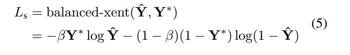
 由于pred_score的结果是经过sigmod得到的,因而取值范围为[0,1],为了避免log计算时的输出为无穷,故log计算中加上极小值np.finfo(np.float32).eps。
case 2
由于分类是对一个个像素点进行分类,通过判断像素点是否在文本框中,那么可以看成语义分割问题,因此部分源码采用Dice Loss。
def get_dice_loss(gt_score, pred_score):
	inter = torch.sum(gt_score * pred_score)
	union = torch.sum(gt_score) + torch.sum(pred_score) + 1e-5
	return 1. - (2 * inter / union)
3.2 几何损失函数
回归损失主要指的是预测框与真实框在几何层面上计算的损失。
(1)对于loc中的d1~d4,并不是计算其与对应标签di的差作为损失,而是根据di计算出预测框与真实框之间的iou来计算损失。iou越大,说明越接近,此时loss应该越小。同时,由于iou取值在[0,1],因此可以将其输入log函数,并乘-1作为loss。

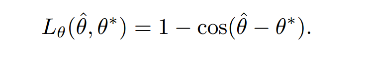
(2)对于angle损失,采用余弦函数,余弦函数的输入为预测angle与真实angle之间的差值,由于是偶函数,故无须对角度差求绝对值。此时角度差越大,cos的输出越小,因此用1-cos的输出作为loss。
3.3 综合损失
根据实际情况,对分类损失、iou loss、angle loss设置不同的系数,进行合并,即为总的损失。
若某个batch中没有正样本(无gtscore),则不计算损失。
def get_dice_loss(gt_score, pred_score):
	inter = torch.sum(gt_score * pred_score)
	union = torch.sum(gt_score) + torch.sum(pred_score) + 1e-5
	return 1. - (2 * inter / union)


def get_geo_loss(gt_geo, pred_geo):
	d1_gt, d2_gt, d3_gt, d4_gt, angle_gt = torch.split(gt_geo, 1, 1)
	d1_pred, d2_pred, d3_pred, d4_pred, angle_pred = torch.split(pred_geo, 1, 1)
	# 真实框的面积
	area_gt = (d1_gt + d2_gt) * (d3_gt + d4_gt)
	# 预测框的面积
	area_pred = (d1_pred + d2_pred) * (d3_pred + d4_pred)
	w_union = torch.min(d3_gt, d3_pred) + torch.min(d4_gt, d4_pred)
	h_union = torch.min(d1_gt, d1_pred) + torch.min(d2_gt, d2_pred)
	area_intersect = w_union * h_union
	area_union = area_gt + area_pred - area_intersect
	# iou损失
	iou_loss_map = -torch.log((area_intersect + 1.0)/(area_union + 1.0))
	# angle损失
	angle_loss_map = 1 - torch.cos(angle_pred - angle_gt)
	return iou_loss_map, angle_loss_map


class Loss(nn.Module):
	def __init__(self, weight_angle=10):
		super(Loss, self).__init__()
		self.weight_angle = weight_angle

	def forward(self, gt_score, pred_score, gt_geo, pred_geo, ignored_map):
		if torch.sum(gt_score) < 1:
			return torch.sum(pred_score + pred_geo) * 0

		classify_loss = get_dice_loss(gt_score, pred_score*(1 - ignored_map))
		iou_loss_map, angle_loss_map = get_geo_loss(gt_geo, pred_geo)
		# 若某个batch中没有正样本(无gtscore),则不计算损失。
		angle_loss = torch.sum(angle_loss_map * gt_score) / torch.sum(gt_score)
		iou_loss = torch.sum(iou_loss_map * gt_score) / torch.sum(gt_score)
		geo_loss = self.weight_angle * angle_loss + iou_loss
		print('classify loss is {:.8f}, angle loss is {:.8f}, iou loss is {:.8f}'.format(classify_loss, angle_loss, iou_loss))
		return geo_loss + classify_loss
4 Advanced EAST
为改进EAST的长文本检测效果不佳的缺陷,有人提出了Advanced EAST,以VGG16作为网络结构的骨干,同样由特征提取层、特征合并层、输出层三部分构成。经实验,Advanced EAST比EAST的检测准确性更好,特别是在长文本上的检测。

4 源码详解
4.1 特征提取层与特征融合层
4.1.1 特征提取层
特征提取层采用了VGG16,总共包含了五组conv block,其中每一组的conv block将通道数变为原来的一倍,并且通过maxpooling的操作,将尺寸变为原图的1/2,(最后一个block通道数不变)。
4.1.2 特征融合层
(1)从最后一个block开始,采用上采样(双线性插值bilinear),将特征图放大一倍。
(2)将放大后的特征图与上一层的特征图concat(通道数叠加)。
(3)利用11卷积核减少concat后的通道数。
(4)最后采用33的卷积核进行特征融合(通道数不变)。
4.1.3 融合部分代码实现
class merge(nn.Module):
	def __init__(self):
		super(merge, self).__init__()

		# 1*1卷积降低维度,1024--->128
		self.conv1 = nn.Conv2d(1024, 128, 1)
		self.bn1 = nn.BatchNorm2d(128)
		self.relu1 = nn.ReLU()
		# 3*3卷积维度不变
		self.conv2 = nn.Conv2d(128, 128, 3, padding=1)
		self.bn2 = nn.BatchNorm2d(128)
		self.relu2 = nn.ReLU()
		# 1*1卷积降低维度,384---->64
		self.conv3 = nn.Conv2d(384, 64, 1)
		self.bn3 = nn.BatchNorm2d(64)
		self.relu3 = nn.ReLU()
		# 3*3卷积维度不变
		self.conv4 = nn.Conv2d(64, 64, 3, padding=1)
		self.bn4 = nn.BatchNorm2d(64)
		self.relu4 = nn.ReLU()
		# 1*1卷积降低维度,192---->32
		self.conv5 = nn.Conv2d(192, 32, 1)
		self.bn5 = nn.BatchNorm2d(32)
		self.relu5 = nn.ReLU()
		# 3*3卷积维度不变
		self.conv6 = nn.Conv2d(32, 32, 3, padding=1)
		self.bn6 = nn.BatchNorm2d(32)
		self.relu6 = nn.ReLU()

		# 3*3卷积维度不变
		self.conv7 = nn.Conv2d(32, 32, 3, padding=1)
		self.bn7 = nn.BatchNorm2d(32)
		self.relu7 = nn.ReLU()

		for m in self.modules():
			if isinstance(m, nn.Conv2d):
				nn.init.kaiming_normal_(m.weight, mode='fan_out', nonlinearity='relu')
				if m.bias is not None:
					nn.init.constant_(m.bias, 0)
			elif isinstance(m, nn.BatchNorm2d):
				nn.init.constant_(m.weight, 1)
				nn.init.constant_(m.bias, 0)

	def forward(self, x):
		# 将输入x[3]进行上采样,上采样的结果为原图的2倍,采样方式为双线性插值,保持角点像素的值
		# 1/32 ---> 1/16
		y = F.interpolate(x[3], scale_factor=2, mode='bilinear', align_corners=True)
		# 将x[3]上采样的结果与x[2]相拼接,其中x[3]的通道数为512, x[2]的通道数也是512
		y = torch.cat((y, x[2]), 1)
		# y的输入通道数 = 512+512=1024, conv1为1*1的卷积核,输出通道数为128
		y = self.relu1(self.bn1(self.conv1(y)))
		# y的输入通道数 = 128, conv2为3*3的卷积核,输出通道数为128
		y = self.relu2(self.bn2(self.conv2(y)))

		# 1/16 ---> 1/8
		y = F.interpolate(y, scale_factor=2, mode='bilinear', align_corners=True)
		# 128 + 256 = 384
		y = torch.cat((y, x[1]), 1)
		# 1*1卷积, 通道数384--->64
		y = self.relu3(self.bn3(self.conv3(y)))
		# 3*3卷积, 通道数为64--->64
		y = self.relu4(self.bn4(self.conv4(y)))

		# 1/8 ---> 1/4
		y = F.interpolate(y, scale_factor=2, mode='bilinear', align_corners=True)
		# 64 + 128 = 192
		y = torch.cat((y, x[0]), 1)
		# 1*1卷积, 通道数192--->32
		y = self.relu5(self.bn5(self.conv5(y)))
		# 3*3卷积, 通道数为32--->32
		y = self.relu6(self.bn6(self.conv6(y)))

		# 3*3卷积, 通道数为32--->32
		y = self.relu7(self.bn7(self.conv7(y)))
		return y
4.2 输出层
输出层主要通过不同的1*1卷积,将特征融合层的结果转换为预测score map、local map所需要的维度。
class output(nn.Module):
	def __init__(self, scope=512):
		super(output, self).__init__()
		# 1*1卷积核,32--->1,获得score map的输出
		self.conv1 = nn.Conv2d(32, 1, 1)
		self.sigmoid1 = nn.Sigmoid()

		# 1*1卷积核,32--->4,获得位置的输出
		self.conv2 = nn.Conv2d(32, 4, 1)
		self.sigmoid2 = nn.Sigmoid()

		# 1*1卷积核,32--->1,获得角度的输出
		self.conv3 = nn.Conv2d(32, 1, 1)
		self.sigmoid3 = nn.Sigmoid()
		# 输入图像的尺寸
		self.scope = 512
		for m in self.modules():
			if isinstance(m, nn.Conv2d):
				nn.init.kaiming_normal_(m.weight, mode='fan_out', nonlinearity='relu')
				if m.bias is not None:
					nn.init.constant_(m.bias, 0)

	def forward(self, x):
		# 利用sigmoid()映射到概率(0~1)
		score = self.sigmoid1(self.conv1(x))
		# loc为d1~d4,输入图像中每点到其所属文本框边界上下左右的距离
		loc   = self.sigmoid2(self.conv2(x)) * self.scope
		# 旋转角的搜索范围是 - π / 2~π / 2
		angle = (self.sigmoid3(self.conv3(x)) - 0.5) * math.pi
		# 合并loc与angle
		geo   = torch.cat((loc, angle), 1)
		return score, geo
5 数据预处理与标签生成
5.1 重载DataSet类
原始的gt格式如下:
764,321,803,317,804,333,763,338,###
1113,374,1178,371,1178,391,1110,398,Supplies
1079,345,1146,338,1148,369,1085,374,WEN
993,378,1033,379,1035,398,998,398,###
1035,377,1074,375,1073,396,1032,401,Globe
1020,349,1081,344,1083,372,1024,376,YONG
其中,前8个数字表示文本框的四个顶点坐标(x,y),最后一个为类别标签,有两类类别标签,第一种是文本内容(如Supplies),第二种是###,###代表忽略这些文本框,不参与计算。
在DataSet类中,主要包含如下操作:
(1) 图像的样本增强
a.随机缩放高度至[0.8–1.2]
b.旋转角度 [-10, 10]
c.随机裁剪512*512的图片
d.改变亮度、对比度、饱和度
(2)获得score_map、geo_map、ignored_map
score_map:每个点是否属于文本框,0或1
geo_map:d1~d4(每个点到文本框的边界距离)和angle(文本框和水平轴夹角)
ignored_map:标签为‘###’的点对应的坐标
class custom_dataset(data.Dataset):
	def __init__(self, img_path, gt_path, scale=0.25, length=512):
		super(custom_dataset, self).__init__()
		# 训练集图像文件与标签文件路径
		self.img_files = [os.path.join(img_path, img_file) for img_file in sorted(os.listdir(img_path))]
		self.gt_files  = [os.path.join(gt_path, gt_file) for gt_file in sorted(os.listdir(gt_path))]
		# 缩放比例,输出的特征图为输入图像的1/4
		self.scale = scale
		# 输入图像的边长,512,即输入图像大小512*512
		self.length = length

	def __len__(self):
		return len(self.img_files)

	def __getitem__(self, index):
		with open(self.gt_files[index], 'r') as f:
			lines = f.readlines()

		# 从gt文本中解析出文本框的四个顶点坐标和类别标签
		# vertices:8维,表示bbox四个顶点的(x,y)坐标
		# labels:1维,表示类别标签,类别标签为文本内容或‘###’其中‘###’代表忽略这些文本框,不参与计算
		vertices, labels = extract_vertices(lines)

		# 图像的样本增强
		img = Image.open(self.img_files[index])
		# 随机缩放高度[0.8--1.2]
		img, vertices = adjust_height(img, vertices)
		# 旋转角度 [-10, 10]
		img, vertices = rotate_img(img, vertices)
		# 随机裁剪512*512的图片
		img, vertices = crop_img(img, vertices, labels, self.length)
		# 改变亮度、对比度、饱和度
		transform = transforms.Compose([transforms.ColorJitter(0.5, 0.5, 0.5, 0.25), \
                                        transforms.ToTensor(), \
                                        transforms.Normalize(mean=(0.5,0.5,0.5),std=(0.5,0.5,0.5))])
		# score_map:每个点是否属于文本框,0或1
		# geo_map:d1~d4(每个点到文本框的边界距离)和angle(文本框和水平轴夹角)
		# ignored_map:标签为‘###’的点对应的坐标
		score_map, geo_map, ignored_map = get_score_geo(img, vertices, labels, self.scale, self.length)
		return transform(img), score_map, geo_map, ignored_map
5.2 crop_img
crop_img主要执行以下操作:
(1)将短边放大至512,长边则根据短边放大的比例进行放大。
(2)根据缩放比例,求取缩放后四个顶点的坐标。
(3)在放缩后多出的空间里,随机选取切割后的左上角起点。
(4)循环1000次,直到裁剪时不会割裂图像中的任一文本框。
(5)找到最终裁剪方案,进行图像裁剪。
(6)根据裁剪后的结果,移动文本框的顶点坐标。
def crop_img(img, vertices, labels, length):
	h, w = img.height, img.width
	# 如果短边 < 512 ,将短边放大到512,另一边等比例放大
	if h >= w and w < length:
		img = img.resize((length, int(h * length / w)), Image.BILINEAR)
	elif h < w and h < length:
		img = img.resize((int(w * length / h), length), Image.BILINEAR)
	# 缩放后的宽高相当于原来的比例
	ratio_w = img.width / w
	ratio_h = img.height / h
	assert(ratio_w >= 1 and ratio_h >= 1)
	# 缩放四个顶点坐标
	new_vertices = np.zeros(vertices.shape)
	if vertices.size > 0:
		new_vertices[:,[0,2,4,6]] = vertices[:,[0,2,4,6]] * ratio_w
		new_vertices[:,[1,3,5,7]] = vertices[:,[1,3,5,7]] * ratio_h

	# 缩放后的图像宽高相对于512*512大小多出的空间
	remain_h = img.height - length
	remain_w = img.width - length
	flag = True
	cnt = 0

	#进行最多1000次随机裁剪,直到找到符合要求的方案
	while flag and cnt < 1000:
		cnt += 1
		start_w = int(np.random.rand() * remain_w)
		start_h = int(np.random.rand() * remain_h)
		# 判断裁剪是否符合要求,即是否割裂图中的文本框
		flag = is_cross_text([start_w, start_h], length, new_vertices[labels==1,:])
	# 找到最终裁剪方案,进行图像裁剪,box为最终裁剪的结果区域
	box = (start_w, start_h, start_w + length, start_h + length)
	region = img.crop(box)
	if new_vertices.size == 0:
		return region, new_vertices
	# 根据裁剪后的结果,移动文本框的顶点坐标
	new_vertices[:,[0,2,4,6]] -= start_w
	new_vertices[:,[1,3,5,7]] -= start_h
	return region, new_vertices
5.3 get_score_geo
这部分主要用于生成score_map、geo_map、ignored_map。具体步骤如下:
(1)新建输入图像1/4尺寸大小的score_map、geo_map、ignored_map。
(2)遍历文本框vertice数组的顶点,给geo_map赋值
(3)将文本框内缩
(4)旋转文本框至水平状态,求水平状态下的顶点坐标。
(5)对旋转后的图像每点(包括框外的)计算d。
(6)填充ignored_map
(7)填充score_map
def get_score_geo(img, vertices, labels, scale, length):
	'''generate score gt and geometry gt
	Input:
		img     : PIL Image
		vertices: vertices of text regions <numpy.ndarray, (n,8)>
		labels  : 1->valid, 0->ignore, <numpy.ndarray, (n,)>
		scale   : feature map / image
		length  : image length
	Output:
		score gt, geo gt, ignored
	'''
	# scale = 1/4,map的尺寸为输入图像的1/4
	score_map   = np.zeros((int(img.height * scale), int(img.width * scale), 1), np.float32)
	geo_map     = np.zeros((int(img.height * scale), int(img.width * scale), 5), np.float32)
	ignored_map = np.zeros((int(img.height * scale), int(img.width * scale), 1), np.float32)
	# 在输入图像上每隔4个点进行下采样,使其和最终特征图的尺寸一致
	index = np.arange(0, length, int(1/scale))
	index_x, index_y = np.meshgrid(index, index)

	ignored_polys = []
	polys = []

	# 遍历顶点,给geo_map赋值
	for i, vertice in enumerate(vertices):
		# 记录需要忽略的四边形
		if labels[i] == 0:
			ignored_polys.append(np.around(scale * vertice.reshape((4,2))).astype(np.int32))
			continue
		# 将文本框内缩,按照1/4下采样缩小
		poly = np.around(scale * shrink_poly(vertice).reshape((4,2))).astype(np.int32) # scaled & shrinked
		polys.append(poly)
		# 单个框的掩码,限定d1,d2,d3,d4中哪些位置应该赋值
		temp_mask = np.zeros(score_map.shape[:-1], np.float32)
		cv2.fillPoly(temp_mask, [poly], 1)
		# 通过遍历,找到最小外接矩形
		theta = find_min_rect_angle(vertice)
		# 旋转文本框至水平状态,便于计算d
		rotate_mat = get_rotate_mat(theta)
		# 旋转文本框四个顶点的坐标至水平状态
		rotated_vertices = rotate_vertices(vertice, theta)
		x_min, x_max, y_min, y_max = get_boundary(rotated_vertices)
		rotated_x, rotated_y = rotate_all_pixels(rotate_mat, vertice[0], vertice[1], length)
		# 对旋转后的图像每点(包括框外的)计算d
		d1 = rotated_y - y_min
		d1[d1<0] = 0
		d2 = y_max - rotated_y
		d2[d2<0] = 0
		d3 = rotated_x - x_min
		d3[d3<0] = 0
		d4 = x_max - rotated_x
		d4[d4<0] = 0
		geo_map[:,:,0] += d1[index_y, index_x] * temp_mask
		geo_map[:,:,1] += d2[index_y, index_x] * temp_mask
		geo_map[:,:,2] += d3[index_y, index_x] * temp_mask
		geo_map[:,:,3] += d4[index_y, index_x] * temp_mask
		geo_map[:,:,4] += theta * temp_mask
	# 填充ignored_map
	cv2.fillPoly(ignored_map, ignored_polys, 1)
	# 填充score_map
	cv2.fillPoly(score_map, polys, 1)
	return torch.Tensor(score_map).permute(2,0,1), torch.Tensor(geo_map).permute(2,0,1), torch.Tensor(ignored_map).permute(2,0,1)
5.4 locality_aware_nms
nms部分采用了局部感知的非极大值抑制,局部感知的 NMS 的不同之处在于对于两个框,在它们的 IoU 大于阀值的时候,不是直接去掉一个,而是将它们进行合并。


 6179
6179


 被折叠的 条评论
为什么被折叠?
被折叠的 条评论
为什么被折叠?
 到【灌水乐园】发言


