


小白学Pytorch系列–Torch API (9)

Other Operations
atleast_1d
返回每个零维输入张量的一维视图。具有一个或多个维度的输入张量将按原样返回。

>>> x = torch.arange(2)
>>> x
tensor([0, 1])
>>> torch.atleast_1d(x)
tensor([0, 1])
>>> x = torch.tensor(1.)
>>> x
tensor(1.)
>>> torch.atleast_1d(x)
tensor([1.])
>>> x = torch.tensor(0.5)
>>> y = torch.tensor(1.)
>>> torch.atleast_1d((x, y))
(tensor([0.5000]), tensor([1.]))
atleast_2d
返回每个零维输入张量的二维视图。具有两个或更多维度的输入张量将按原样返回。

>>> x = torch.tensor(1.)
>>> x
tensor(1.)
>>> torch.atleast_2d(x)
tensor([[1.]])
>>> x = torch.arange(4).view(2, 2)
>>> x
tensor([[0, 1],
        [2, 3]])
>>> torch.atleast_2d(x)
tensor([[0, 1],
        [2, 3]])
>>> x = torch.tensor(0.5)
>>> y = torch.tensor(1.)
>>> torch.atleast_2d((x, y))
(tensor([[0.5000]]), tensor([[1.]]))
atleast_3d
返回每个零维输入张量的三维视图。具有三维或三维以上维度的输入张量将按原样返回。

>>> x = torch.tensor(0.5)
>>> x
tensor(0.5000)
>>> torch.atleast_3d(x)
tensor([[[0.5000]]])
>>> y = torch.arange(4).view(2, 2)
>>> y
tensor([[0, 1],
        [2, 3]])
>>> torch.atleast_3d(y)
tensor([[[0],
         [1]],

        [[2],
         [3]]])
>>> x = torch.tensor(1).view(1, 1, 1)
>>> x
tensor([[[1]]])
>>> torch.atleast_3d(x)
tensor([[[1]]])
>>> x = torch.tensor(0.5)
>>> y = torch.tensor(1.)
>>> torch.atleast_3d((x, y))
(tensor([[[0.5000]]]), tensor([[[1.]]]))
bincount
计算非负整数数组中每个值的频率。
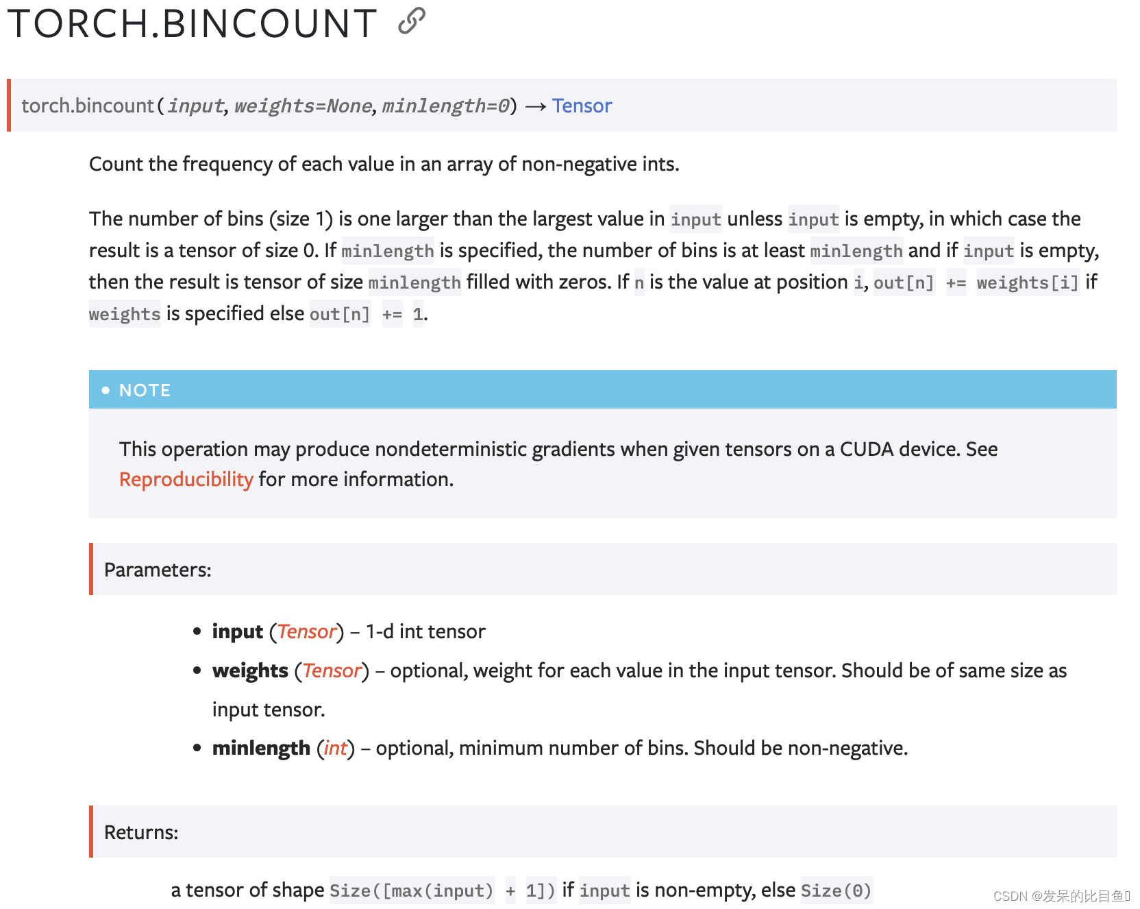
>>> input = torch.randint(0, 8, (5,), dtype=torch.int64)
>>> weights = torch.linspace(0, 1, steps=5)
>>> input, weights
(tensor([4, 3, 6, 3, 4]),
 tensor([ 0.0000,  0.2500,  0.5000,  0.7500,  1.0000])

>>> torch.bincount(input)
tensor([0, 0, 0, 2, 2, 0, 1])

>>> input.bincount(weights)
tensor([0.0000, 0.0000, 0.0000, 1.0000, 1.0000, 0.0000, 0.5000])
block_diag
根据提供的张量创建块对角矩阵。

>>> import torch
>>> A = torch.tensor([[0, 1], [1, 0]])
>>> B = torch.tensor([[3, 4, 5], [6, 7, 8]])
>>> C = torch.tensor(7)
>>> D = torch.tensor([1, 2, 3])
>>> E = torch.tensor([[4], [5], [6]])
>>> torch.block_diag(A, B, C, D, E)
tensor([[0, 1, 0, 0, 0, 0, 0, 0, 0, 0],
        [1, 0, 0, 0, 0, 0, 0, 0, 0, 0],
        [0, 0, 3, 4, 5, 0, 0, 0, 0, 0],
        [0, 0, 6, 7, 8, 0, 0, 0, 0, 0],
        [0, 0, 0, 0, 0, 7, 0, 0, 0, 0],
        [0, 0, 0, 0, 0, 0, 1, 2, 3, 0],
        [0, 0, 0, 0, 0, 0, 0, 0, 0, 4],
        [0, 0, 0, 0, 0, 0, 0, 0, 0, 5],
        [0, 0, 0, 0, 0, 0, 0, 0, 0, 6]])
broadcast_tensors
根据广播语义广播给定的张量。
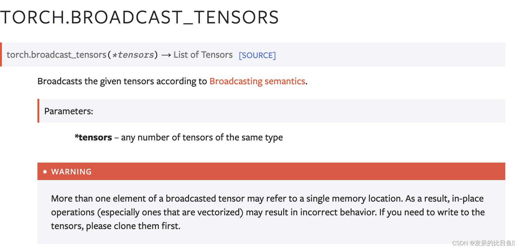
>>> x = torch.arange(3).view(1, 3)
>>> y = torch.arange(2).view(2, 1)
>>> a, b = torch.broadcast_tensors(x, y)
>>> a.size()
torch.Size([2, 3])
>>> a
tensor([[0, 1, 2],
        [0, 1, 2]])
broadcast_to
将输入广播到形状。相当于调用input.expand(shape)。有关详细信息,请参阅expand()。

>>> x = torch.tensor([1, 2, 3])
>>> torch.broadcast_to(x, (3, 3))
tensor([[1, 2, 3],
        [1, 2, 3],
        [1, 2, 3]])
broadcast_shapes
类似于broadcast_tensors() 用于形状。

>>> torch.broadcast_shapes((2,), (3, 1), (1, 1, 1))
torch.Size([1, 3, 2])
bucketize
返回输入中每个值所属的存储桶的索引,其中存储桶的边界由边界设置。返回一个与输入大小相同的新张量。如果right为False(默认值),则关闭左侧边界。更正式地说,返回的索引满足以下规则:

>>> boundaries = torch.tensor([1, 3, 5, 7, 9])
>>> boundaries
tensor([1, 3, 5, 7, 9])
>>> v = torch.tensor([[3, 6, 9], [3, 6, 9]])
>>> v
tensor([[3, 6, 9],
        [3, 6, 9]])
>>> torch.bucketize(v, boundaries)
tensor([[1, 3, 4],
        [1, 3, 4]])
>>> torch.bucketize(v, boundaries, right=True)
tensor([[2, 3, 5],
        [2, 3, 5]])
cartesian_prod
做给定张量序列的笛卡尔乘积。该行为类似于python的itertools.product。

>>> import itertools
>>> a = [1, 2, 3]
>>> b = [4, 5]
>>> list(itertools.product(a, b))
[(1, 4), (1, 5), (2, 4), (2, 5), (3, 4), (3, 5)]
>>> tensor_a = torch.tensor(a)
>>> tensor_b = torch.tensor(b)
>>> torch.cartesian_prod(tensor_a, tensor_b)
tensor([[1, 4],
        [1, 5],
        [2, 4],
        [2, 5],
        [3, 4],
        [3, 5]])
cdist
批量计算两个行向量集合的每对之间的p范数距离。

>>> a = torch.tensor([[0.9041,  0.0196], [-0.3108, -2.4423], [-0.4821,  1.059]])
>>> a
tensor([[ 0.9041,  0.0196],
        [-0.3108, -2.4423],
        [-0.4821,  1.0590]])
>>> b = torch.tensor([[-2.1763, -0.4713], [-0.6986,  1.3702]])
>>> b
tensor([[-2.1763, -0.4713],
        [-0.6986,  1.3702]])
>>> torch.cdist(a, b, p=2)
tensor([[3.1193, 2.0959],
        [2.7138, 3.8322],
        [2.2830, 0.3791]])
clone
返回输入的副本。

combinations
计算给定张量的长度r的组合。当with_replacement设置为False时,该行为类似于python的itertools.combinations,当with_relacement设置为True时,其行为类似于itertool.combinations_with_replacement。

>>> a = [1, 2, 3]
>>> list(itertools.combinations(a, r=2))
[(1, 2), (1, 3), (2, 3)]
>>> list(itertools.combinations(a, r=3))
[(1, 2, 3)]
>>> list(itertools.combinations_with_replacement(a, r=2))
[(1, 1), (1, 2), (1, 3), (2, 2), (2, 3), (3, 3)]
>>> tensor_a = torch.tensor(a)
>>> torch.combinations(tensor_a)
tensor([[1, 2],
        [1, 3],
        [2, 3]])
>>> torch.combinations(tensor_a, r=3)
tensor([[1, 2, 3]])
>>> torch.combinations(tensor_a, with_replacement=True)
tensor([[1, 1],
        [1, 2],
        [1, 3],
        [2, 2],
        [2, 3],
        [3, 3]])
corrcoef
估计输入矩阵给出的变量的皮尔逊乘积矩相关系数矩阵,其中行是变量,列是观测值。

>>> x = torch.tensor([[0, 1, 2], [2, 1, 0]])
>>> torch.corrcoef(x)
tensor([[ 1., -1.],
        [-1.,  1.]])
>>> x = torch.randn(2, 4)
>>> x
tensor([[-0.2678, -0.0908, -0.3766,  0.2780],
        [-0.5812,  0.1535,  0.2387,  0.2350]])
>>> torch.corrcoef(x)
tensor([[1.0000, 0.3582],
        [0.3582, 1.0000]])
>>> torch.corrcoef(x[0])
tensor(1.)
cov
估计输入矩阵给出的变量的协方差矩阵,其中行是变量,列是观测值。


>>> x = torch.tensor([[0, 2], [1, 1], [2, 0]]).T
>>> x
tensor([[0, 1, 2],
        [2, 1, 0]])
>>> torch.cov(x)
tensor([[ 1., -1.],
        [-1.,  1.]])
>>> torch.cov(x, correction=0)
tensor([[ 0.6667, -0.6667],
        [-0.6667,  0.6667]])
>>> fw = torch.randint(1, 10, (3,))
>>> fw
tensor([1, 6, 9])
>>> aw = torch.rand(3)
>>> aw
tensor([0.4282, 0.0255, 0.4144])
>>> torch.cov(x, fweights=fw, aweights=aw)
tensor([[ 0.4169, -0.4169],
        [-0.4169,  0.4169]])
cross
返回输入和其他维度dim中向量的叉积。即两个向量面的垂直向量。
支持float、double、cfloat和cddouble数据类型的输入。还支持向量的批处理,为其计算沿维度dim的乘积。在这种情况下,输出具有与输入相同的批次维度。
如果未给定dim,则默认为大小为3的第一个维度。请注意,这可能是出乎意料的。


>>> a = torch.randn(4, 3)
>>> a
tensor([[-0.3956,  1.1455,  1.6895],
        [-0.5849,  1.3672,  0.3599],
        [-1.1626,  0.7180, -0.0521],
        [-0.1339,  0.9902, -2.0225]])
>>> b = torch.randn(4, 3)
>>> b
tensor([[-0.0257, -1.4725, -1.2251],
        [-1.1479, -0.7005, -1.9757],
        [-1.3904,  0.3726, -1.1836],
        [-0.9688, -0.7153,  0.2159]])
>>> torch.cross(a, b, dim=1)
tensor([[ 1.0844, -0.5281,  0.6120],
        [-2.4490, -1.5687,  1.9792],
        [-0.8304, -1.3037,  0.5650],
        [-1.2329,  1.9883,  1.0551]])
>>> torch.cross(a, b)
tensor([[ 1.0844, -0.5281,  0.6120],
        [-2.4490, -1.5687,  1.9792],
        [-0.8304, -1.3037,  0.5650],
        [-1.2329,  1.9883,  1.0551]])
cummax
返回一个命名元组(值、索引),其中值是维度dim中输入元素的累积最大值。索引是在维度dim中找到的每个最大值的索引位置。
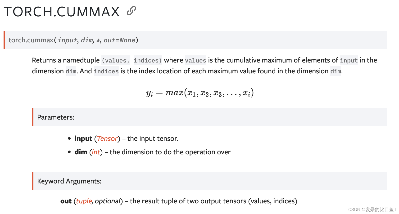
>>> a = torch.randn(10)
>>> a
tensor([-0.3449, -1.5447,  0.0685, -1.5104, -1.1706,  0.2259,  1.4696, -1.3284,
     1.9946, -0.8209])
>>> torch.cummax(a, dim=0)
torch.return_types.cummax(
    values=tensor([-0.3449, -0.3449,  0.0685,  0.0685,  0.0685,  0.2259,  1.4696,  1.4696,
     1.9946,  1.9946]),
    indices=tensor([0, 0, 2, 2, 2, 5, 6, 6, 8, 8]))
cummin
返回一个命名元组(值、索引),其中值是维度dim中输入元素的累积最小值。索引是在维度dim中找到的每个最大值的索引位置。

>>> a = torch.randn(10)
>>> a
tensor([-0.2284, -0.6628,  0.0975,  0.2680, -1.3298, -0.4220, -0.3885,  1.1762,
     0.9165,  1.6684])
>>> torch.cummin(a, dim=0)
torch.return_types.cummin(
    values=tensor([-0.2284, -0.6628, -0.6628, -0.6628, -1.3298, -1.3298, -1.3298, -1.3298,
    -1.3298, -1.3298]),
    indices=tensor([0, 1, 1, 1, 4, 4, 4, 4, 4, 4]))
cumprod
返回维度dim中输入元素的累积乘积。
例如,如果输入是大小为N的向量,则结果也将是大小为N的向量,其中包含元素。

>>> a = torch.randn(10)
>>> a
tensor([ 0.6001,  0.2069, -0.1919,  0.9792,  0.6727,  1.0062,  0.4126,
        -0.2129, -0.4206,  0.1968])
>>> torch.cumprod(a, dim=0)
tensor([ 0.6001,  0.1241, -0.0238, -0.0233, -0.0157, -0.0158, -0.0065,
         0.0014, -0.0006, -0.0001])

>>> a[5] = 0.0
>>> torch.cumprod(a, dim=0)
tensor([ 0.6001,  0.1241, -0.0238, -0.0233, -0.0157, -0.0000, -0.0000,
         0.0000, -0.0000, -0.0000])
cumsum
返回维度dim中输入元素的累积和。
例如,如果输入是大小为N的向量,则结果也将是大小为N的向量,其中包含元素。

>>> a = torch.randn(10)
>>> a
tensor([-0.8286, -0.4890,  0.5155,  0.8443,  0.1865, -0.1752, -2.0595,
         0.1850, -1.1571, -0.4243])
>>> torch.cumsum(a, dim=0)
tensor([-0.8286, -1.3175, -0.8020,  0.0423,  0.2289,  0.0537, -2.0058,
        -1.8209, -2.9780, -3.4022])
diag
得到输入向量为对角线的方阵

>>> a = torch.randn(3)
>>> a
tensor([ 0.5950,-0.0872, 2.3298])
>>> torch.diag(a)
tensor([[ 0.5950, 0.0000, 0.0000],
        [ 0.0000,-0.0872, 0.0000],
        [ 0.0000, 0.0000, 2.3298]])
>>> torch.diag(a, 1)
tensor([[ 0.0000, 0.5950, 0.0000, 0.0000],
        [ 0.0000, 0.0000,-0.0872, 0.0000],
        [ 0.0000, 0.0000, 0.0000, 2.3298],
        [ 0.0000, 0.0000, 0.0000, 0.0000]])
求给定矩阵的第k个对角线
>>> a = torch.randn(3, 3)
>>> a
tensor([[-0.4264, 0.0255,-0.1064],
        [ 0.8795,-0.2429, 0.1374],
        [ 0.1029,-0.6482,-1.6300]])
>>> torch.diag(a, 0)
tensor([-0.4264,-0.2429,-1.6300])
>>> torch.diag(a, 1)
tensor([ 0.0255, 0.1374])
diag_embed
创建一个张量,其某些二维平面(由dim1和dim2指定)的对角线由输入填充。为了便于创建批量对角矩阵,默认情况下选择由返回张量的最后两个维度形成的2D平面。
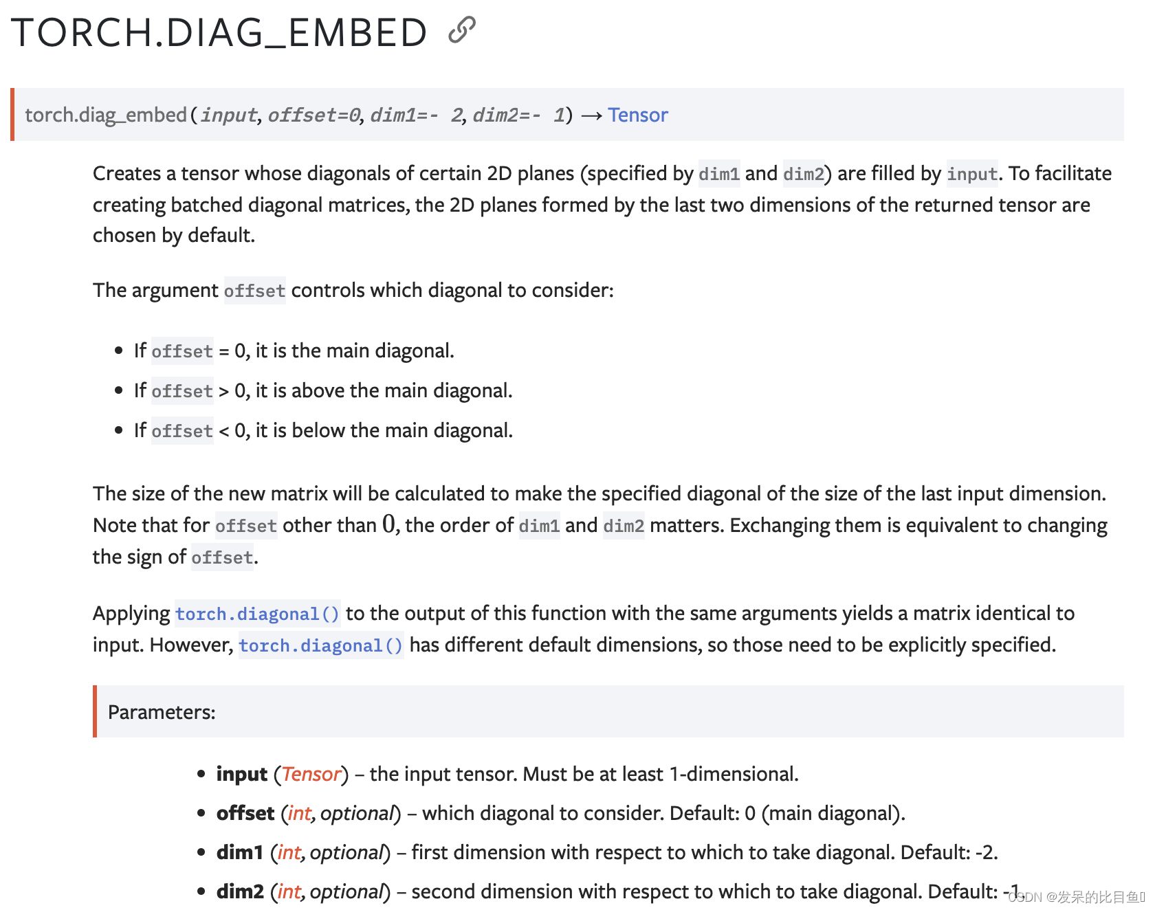
>>> a = torch.randn(2, 3)
>>> torch.diag_embed(a)
tensor([[[ 1.5410,  0.0000,  0.0000],
         [ 0.0000, -0.2934,  0.0000],
         [ 0.0000,  0.0000, -2.1788]],

        [[ 0.5684,  0.0000,  0.0000],
         [ 0.0000, -1.0845,  0.0000],
         [ 0.0000,  0.0000, -1.3986]]])

>>> torch.diag_embed(a, offset=1, dim1=0, dim2=2)
tensor([[[ 0.0000,  1.5410,  0.0000,  0.0000],
         [ 0.0000,  0.5684,  0.0000,  0.0000]],

        [[ 0.0000,  0.0000, -0.2934,  0.0000],
         [ 0.0000,  0.0000, -1.0845,  0.0000]],

        [[ 0.0000,  0.0000,  0.0000, -2.1788],
         [ 0.0000,  0.0000,  0.0000, -1.3986]],

        [[ 0.0000,  0.0000,  0.0000,  0.0000],
         [ 0.0000,  0.0000,  0.0000,  0.0000]]])
diagflat

>>> a = torch.randn(3)
>>> a
tensor([-0.2956, -0.9068,  0.1695])
>>> torch.diagflat(a)
tensor([[-0.2956,  0.0000,  0.0000],
        [ 0.0000, -0.9068,  0.0000],
        [ 0.0000,  0.0000,  0.1695]])
>>> torch.diagflat(a, 1)
tensor([[ 0.0000, -0.2956,  0.0000,  0.0000],
        [ 0.0000,  0.0000, -0.9068,  0.0000],
        [ 0.0000,  0.0000,  0.0000,  0.1695],
        [ 0.0000,  0.0000,  0.0000,  0.0000]])

>>> a = torch.randn(2, 2)
>>> a
tensor([[ 0.2094, -0.3018],
        [-0.1516,  1.9342]])
>>> torch.diagflat(a)
tensor([[ 0.2094,  0.0000,  0.0000,  0.0000],
        [ 0.0000, -0.3018,  0.0000,  0.0000],
        [ 0.0000,  0.0000, -0.1516,  0.0000],
        [ 0.0000,  0.0000,  0.0000,  1.9342]])
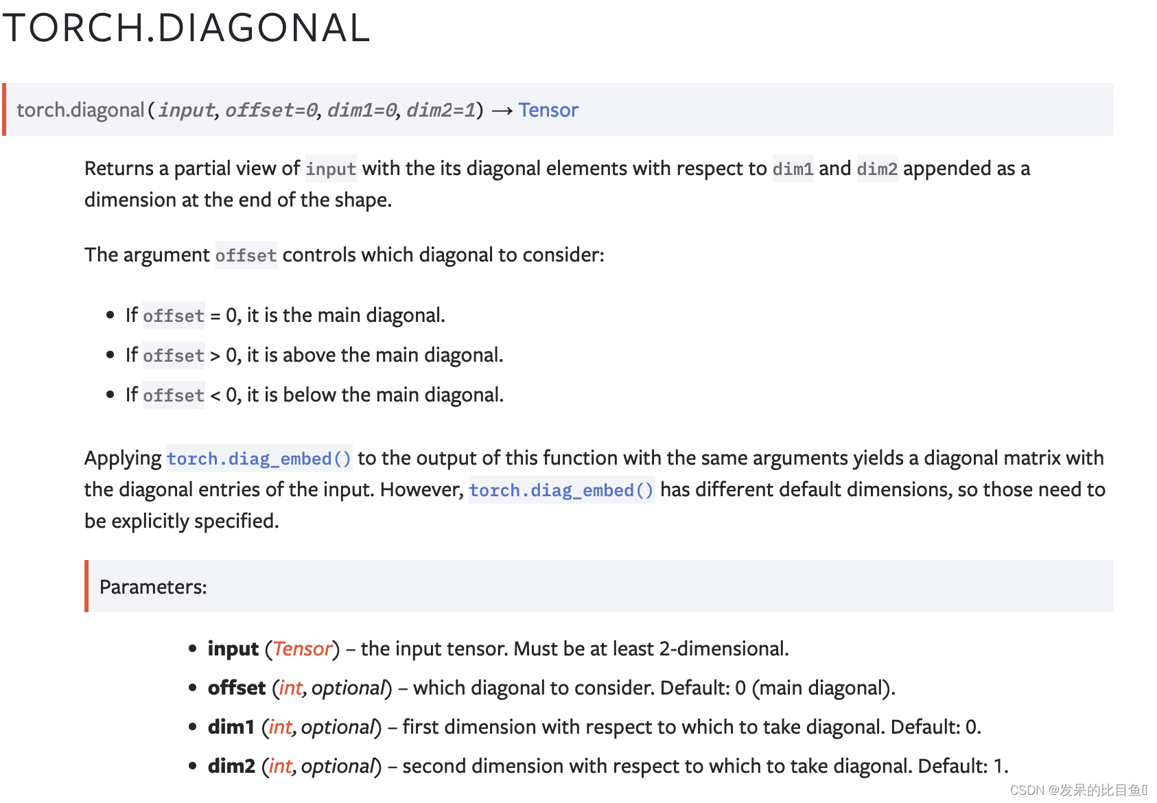
diagonal
返回输入的局部视图,其中包含相对于dim1和dim2的对角元素,并将其附加为形状末尾的维度。
>>> a = torch.randn(3, 3)
>>> a
tensor([[-1.0854,  1.1431, -0.1752],
        [ 0.8536, -0.0905,  0.0360],
        [ 0.6927, -0.3735, -0.4945]])


>>> torch.diagonal(a, 0)
tensor([-1.0854, -0.0905, -0.4945])


>>> torch.diagonal(a, 1)
tensor([ 1.1431,  0.0360])


>>> x = torch.randn(2, 5, 4, 2)
>>> torch.diagonal(x, offset=-1, dim1=1, dim2=2)
tensor([[[-1.2631,  0.3755, -1.5977, -1.8172],
         [-1.1065,  1.0401, -0.2235, -0.7938]],

        [[-1.7325, -0.3081,  0.6166,  0.2335],
         [ 1.0500,  0.7336, -0.3836, -1.1015]]])
diff
计算沿给定维度的第n个正向差。

>>> a = torch.tensor([1, 3, 2])
>>> torch.diff(a)
tensor([ 2, -1])
>>> b = torch.tensor([4, 5])
>>> torch.diff(a, append=b)
tensor([ 2, -1,  2,  1])
>>> c = torch.tensor([[1, 2, 3], [3, 4, 5]])
>>> torch.diff(c, dim=0)
tensor([[2, 2, 2]])
>>> torch.diff(c, dim=1)
tensor([[1, 1],
        [1, 1]])
einsum
求和输入操作数的元素沿着使用基于爱因斯坦求和约定的符号指定的维度的乘积。

>>> # trace
>>> torch.einsum('ii', torch.randn(4, 4))
tensor(-1.2104)

>>> # diagonal
>>> torch.einsum('ii->i', torch.randn(4, 4))
tensor([-0.1034,  0.7952, -0.2433,  0.4545])

>>> # outer product
>>> x = torch.randn(5)
>>> y = torch.randn(4)
>>> torch.einsum('i,j->ij', x, y)
tensor([[ 0.1156, -0.2897, -0.3918,  0.4963],
        [-0.3744,  0.9381,  1.2685, -1.6070],
        [ 0.7208, -1.8058, -2.4419,  3.0936],
        [ 0.1713, -0.4291, -0.5802,  0.7350],
        [ 0.5704, -1.4290, -1.9323,  2.4480]])

>>> # batch matrix multiplication
>>> As = torch.randn(3, 2, 5)
>>> Bs = torch.randn(3, 5, 4)
>>> torch.einsum('bij,bjk->bik', As, Bs)
tensor([[[-1.0564, -1.5904,  3.2023,  3.1271],
        [-1.6706, -0.8097, -0.8025, -2.1183]],

        [[ 4.2239,  0.3107, -0.5756, -0.2354],
        [-1.4558, -0.3460,  1.5087, -0.8530]],

        [[ 2.8153,  1.8787, -4.3839, -1.2112],
        [ 0.3728, -2.1131,  0.0921,  0.8305]]])

>>> # with sublist format and ellipsis
>>> torch.einsum(As, [..., 0, 1], Bs, [..., 1, 2], [..., 0, 2])
tensor([[[-1.0564, -1.5904,  3.2023,  3.1271],
        [-1.6706, -0.8097, -0.8025, -2.1183]],

        [[ 4.2239,  0.3107, -0.5756, -0.2354],
        [-1.4558, -0.3460,  1.5087, -0.8530]],

        [[ 2.8153,  1.8787, -4.3839, -1.2112],
        [ 0.3728, -2.1131,  0.0921,  0.8305]]])

>>> # batch permute
>>> A = torch.randn(2, 3, 4, 5)
>>> torch.einsum('...ij->...ji', A).shape
torch.Size([2, 3, 5, 4])

>>> # equivalent to torch.nn.functional.bilinear
>>> A = torch.randn(3, 5, 4)
>>> l = torch.randn(2, 5)
>>> r = torch.randn(2, 4)
>>> torch.einsum('bn,anm,bm->ba', l, A, r)
tensor([[-0.3430, -5.2405,  0.4494],
        [ 0.3311,  5.5201, -3.0356]])
flatten
通过将输入重塑为一维张量来使其变平。如果传递start_dim或end_dim,则仅展平以start_dim开头和以end_dim结尾的标注。输入中元素的顺序不变。

>>> t = torch.tensor([[[1, 2],
...                    [3, 4]],
...                   [[5, 6],
...                    [7, 8]]])
>>> torch.flatten(t)
tensor([1, 2, 3, 4, 5, 6, 7, 8])
>>> torch.flatten(t, start_dim=1)
tensor([[1, 2, 3, 4],
        [5, 6, 7, 8]])
flip
以dims为单位,沿着给定的轴反转n-D张量的顺序。

>>> x = torch.arange(8).view(2, 2, 2)
>>> x
tensor([[[ 0,  1],
         [ 2,  3]],

        [[ 4,  5],
         [ 6,  7]]])
>>> torch.flip(x, [0, 1])
tensor([[[ 6,  7],
         [ 4,  5]],

        [[ 2,  3],
         [ 0,  1]]])
fliplr

>>> x = torch.arange(4).view(2, 2)
>>> x
tensor([[0, 1],
        [2, 3]])
>>> torch.fliplr(x)
tensor([[1, 0],
        [3, 2]])
flipud
向上/向下翻转张量,返回一个新的张量。
将每列中的条目向上/向下翻转。行被保留,但以与以前不同的顺序显示。

>>> x = torch.arange(4).view(2, 2)
>>> x
tensor([[0, 1],
        [2, 3]])
>>> torch.flipud(x)
tensor([[2, 3],
        [0, 1]])
kron
计算输入和其他的Kronecker乘积,用⊗表示。

>>> mat1 = torch.eye(2)
>>> mat2 = torch.ones(2, 2)
>>> torch.kron(mat1, mat2)
tensor([[1., 1., 0., 0.],
        [1., 1., 0., 0.],
        [0., 0., 1., 1.],
        [0., 0., 1., 1.]])

>>> mat1 = torch.eye(2)
>>> mat2 = torch.arange(1, 5).reshape(2, 2)
>>> torch.kron(mat1, mat2)
tensor([[1., 2., 0., 0.],
        [3., 4., 0., 0.],
        [0., 0., 1., 2.],
        [0., 0., 3., 4.]])
rot90
在dims轴指定的平面中将n-D张量旋转90度。如果k>0,则旋转方向为从第一个轴朝向第二个轴,如果k<0,则从第二个方向朝向第一个轴。

>>> x = torch.arange(4).view(2, 2)
>>> x
tensor([[0, 1],
        [2, 3]])
>>> torch.rot90(x, 1, [0, 1])
tensor([[1, 3],
        [0, 2]])

>>> x = torch.arange(8).view(2, 2, 2)
>>> x
tensor([[[0, 1],
         [2, 3]],

        [[4, 5],
         [6, 7]]])
>>> torch.rot90(x, 1, [1, 2])
tensor([[[1, 3],
         [0, 2]],

        [[5, 7],
         [4, 6]]])
gcd
计算输入和其他的元素最大公约数(GCD)。
输入和其他都必须具有整数类型。

>>> a = torch.tensor([5, 10, 15])
>>> b = torch.tensor([3, 4, 5])
>>> torch.gcd(a, b)
tensor([1, 2, 5])
>>> c = torch.tensor([3])
>>> torch.gcd(a, c)
tensor([1, 1, 3])
histc
计算张量的直方图。
元素被分类到最小值和最大值之间的等宽仓中。如果最小值和最小值都为零,则使用数据的最小值和最高值。
忽略低于最小值且高于最大值的元素和NaN元素。

>>> torch.histc(torch.tensor([1., 2, 1]), bins=4, min=0, max=3)
tensor([ 0.,  2.,  1.,  0.])
histogram
计算张量中值的直方图。

>>> torch.histogram(torch.tensor([1., 2, 1]), bins=4, range=(0., 3.), weight=torch.tensor([1., 2., 4.]))
(tensor([ 0.,  5.,  2.,  0.]), tensor([0., 0.75, 1.5, 2.25, 3.]))
>>> torch.histogram(torch.tensor([1., 2, 1]), bins=4, range=(0., 3.), weight=torch.tensor([1., 2., 4.]), density=True)
(tensor([ 0.,  0.9524,  0.3810,  0.]), tensor([0., 0.75, 1.5, 2.25, 3.]))
histogramdd
计算张量中值的多维直方图。
将最内维度大小为N的输入张量的元素解释为N维点的集合。将每个点映射到一组N维仓中,并返回每个仓中的点数(或总重量)。
输入必须是一个至少有2个维度的张量。如果输入具有形状(M,N),则其M行中的每一行定义N维空间中的一个点。如果输入有三个或多个维度,则除最后一个维度外的所有维度都将被展平。
每个维度都独立地与其自身严格递增的仓边序列相关联。可以通过传递1D张量序列来明确地指定仓边缘。或者,可以通过传递一系列整数来自动构建仓边,这些整数指定每个维度中等宽仓的数量。

>>> torch.histogramdd(torch.tensor([[0., 1.], [1., 0.], [2., 0.], [2., 2.]]), bins=[3, 3],
...                   weight=torch.tensor([1., 2., 4., 8.]))
    torch.return_types.histogramdd(
        hist=tensor([[0., 1., 0.],
                     [2., 0., 0.],
                     [4., 0., 8.]]),
        bin_edges=(tensor([0.0000, 0.6667, 1.3333, 2.0000]),
                   tensor([0.0000, 0.6667, 1.3333, 2.0000])))
>>> torch.histogramdd(torch.tensor([[0., 0.], [1., 1.], [2., 2.]]), bins=[2, 2],
...                   range=[0., 1., 0., 1.], density=True)
    torch.return_types.histogramdd(
       hist=tensor([[2., 0.],
                    [0., 2.]]),
       bin_edges=(tensor([0.0000, 0.5000, 1.0000]),
                  tensor([0.0000, 0.5000, 1.0000])))
meshgrid
创建由属性:张量中的1D输入指定的坐标网格。


>>> x = torch.tensor([1, 2, 3])
>>> y = torch.tensor([4, 5, 6])

Observe the element-wise pairings across the grid, (1, 4),
(1, 5), ..., (3, 6). This is the same thing as the
cartesian product.
>>> grid_x, grid_y = torch.meshgrid(x, y, indexing='ij')
>>> grid_x
tensor([[1, 1, 1],
        [2, 2, 2],
        [3, 3, 3]])
>>> grid_y
tensor([[4, 5, 6],
        [4, 5, 6],
        [4, 5, 6]])

This correspondence can be seen when these grids are
stacked properly.
>>> torch.equal(torch.cat(tuple(torch.dstack([grid_x, grid_y]))),
...             torch.cartesian_prod(x, y))
True

`torch.meshgrid` is commonly used to produce a grid for
plotting.
>>> import matplotlib.pyplot as plt
>>> xs = torch.linspace(-5, 5, steps=100)
>>> ys = torch.linspace(-5, 5, steps=100)
>>> x, y = torch.meshgrid(xs, ys, indexing='xy')
>>> z = torch.sin(torch.sqrt(x * x + y * y))
>>> ax = plt.axes(projection='3d')
>>> ax.plot_surface(x.numpy(), y.numpy(), z.numpy())
>>> plt.show()
lcm
计算输入和其他的元素最小公倍数(LCM)。
输入和其他都必须具有整数类型。

>>> a = torch.tensor([5, 10, 15])
>>> b = torch.tensor([3, 4, 5])
>>> torch.lcm(a, b)
tensor([15, 20, 15])
>>> c = torch.tensor([3])
>>> torch.lcm(a, c)
tensor([15, 30, 15])
logcumsumexp
返回维度dim中输入元素的幂的累积求和的对数。
对于由dim和其他指数i给出的求和指数j,结果是

>>> a = torch.randn(10)
>>> torch.logcumsumexp(a, dim=0)
tensor([-0.42296738, -0.04462666,  0.86278635,  0.94622083,  1.05277811,
         1.39202815,  1.83525007,  1.84492621,  2.06084887,  2.06844475]))
ravel
返回一个连续的扁平张量。只有在需要时才会制作副本。

>>> t = torch.tensor([[[1, 2],
...                    [3, 4]],
...                   [[5, 6],
...                    [7, 8]]])
>>> torch.ravel(t)
tensor([1, 2, 3, 4, 5, 6, 7, 8])
renorm
返回一个张量,其中沿维度dim输入的每个子张量被归一化,使得子张量的p范数低于值maxnorm

>>> x = torch.ones(3, 3)
>>> x[1].fill_(2)
tensor([ 2.,  2.,  2.])
>>> x[2].fill_(3)
tensor([ 3.,  3.,  3.])
>>> x
tensor([[ 1.,  1.,  1.],
        [ 2.,  2.,  2.],
        [ 3.,  3.,  3.]])
>>> torch.renorm(x, 1, 0, 5)
tensor([[ 1.0000,  1.0000,  1.0000],
        [ 1.6667,  1.6667,  1.6667],
        [ 1.6667,  1.6667,  1.6667]])
repeat_interleave
重复张量的元素。

>>> x = torch.tensor([1, 2, 3])
>>> x.repeat_interleave(2)
tensor([1, 1, 2, 2, 3, 3])
>>> y = torch.tensor([[1, 2], [3, 4]])
>>> torch.repeat_interleave(y, 2)
tensor([1, 1, 2, 2, 3, 3, 4, 4])
>>> torch.repeat_interleave(y, 3, dim=1)
tensor([[1, 1, 1, 2, 2, 2],
        [3, 3, 3, 4, 4, 4]])
>>> torch.repeat_interleave(y, torch.tensor([1, 2]), dim=0)
tensor([[1, 2],
        [3, 4],
        [3, 4]])
>>> torch.repeat_interleave(y, torch.tensor([1, 2]), dim=0, output_size=3)
tensor([[1, 2],
        [3, 4],
        [3, 4]])
roll
沿着给定的维度滚动张量输入。移动到最后一个位置之外的元素将在第一个位置重新引入。如果dims为None,则张量将在滚动之前被展平,然后恢复到原始形状。

>>> x = torch.tensor([1, 2, 3, 4, 5, 6, 7, 8]).view(4, 2)
>>> x
tensor([[1, 2],
        [3, 4],
        [5, 6],
        [7, 8]])
>>> torch.roll(x, 1)
tensor([[8, 1],
        [2, 3],
        [4, 5],
        [6, 7]])
>>> torch.roll(x, 1, 0)
tensor([[7, 8],
        [1, 2],
        [3, 4],
        [5, 6]])
>>> torch.roll(x, -1, 0)
tensor([[3, 4],
        [5, 6],
        [7, 8],
        [1, 2]])
>>> torch.roll(x, shifts=(2, 1), dims=(0, 1))
tensor([[6, 5],
        [8, 7],
        [2, 1],
        [4, 3]])
searchsorted
从sorted_sequence的最内层维度中查找索引,这样,如果值中的相应值被插入索引之前,则在排序时,sorted-sequence中相应最内层维度的顺序将被保留。返回一个大小与值相同的新张量。如果right为False或side为’left(默认值),则sorted_sequence的左边界关闭。更正式地说,返回的索引满足以下规则:

>>> sorted_sequence = torch.tensor([[1, 3, 5, 7, 9], [2, 4, 6, 8, 10]])
>>> sorted_sequence
tensor([[ 1,  3,  5,  7,  9],
        [ 2,  4,  6,  8, 10]])
>>> values = torch.tensor([[3, 6, 9], [3, 6, 9]])
>>> values
tensor([[3, 6, 9],
        [3, 6, 9]])
>>> torch.searchsorted(sorted_sequence, values)
tensor([[1, 3, 4],
        [1, 2, 4]])
>>> torch.searchsorted(sorted_sequence, values, side='right')
tensor([[2, 3, 5],
        [1, 3, 4]])

>>> sorted_sequence_1d = torch.tensor([1, 3, 5, 7, 9])
>>> sorted_sequence_1d
tensor([1, 3, 5, 7, 9])
>>> torch.searchsorted(sorted_sequence_1d, values)
tensor([[1, 3, 4],
        [1, 3, 4]])
tensordot
返回a和b在多个维度上的收缩。

>>> a = torch.arange(60.).reshape(3, 4, 5)
>>> b = torch.arange(24.).reshape(4, 3, 2)
>>> torch.tensordot(a, b, dims=([1, 0], [0, 1]))
tensor([[4400., 4730.],
        [4532., 4874.],
        [4664., 5018.],
        [4796., 5162.],
        [4928., 5306.]])

>>> a = torch.randn(3, 4, 5, device='cuda')
>>> b = torch.randn(4, 5, 6, device='cuda')
>>> c = torch.tensordot(a, b, dims=2).cpu()
tensor([[ 8.3504, -2.5436,  6.2922,  2.7556, -1.0732,  3.2741],
        [ 3.3161,  0.0704,  5.0187, -0.4079, -4.3126,  4.8744],
        [ 0.8223,  3.9445,  3.2168, -0.2400,  3.4117,  1.7780]])

>>> a = torch.randn(3, 5, 4, 6)
>>> b = torch.randn(6, 4, 5, 3)
>>> torch.tensordot(a, b, dims=([2, 1, 3], [1, 2, 0]))
tensor([[  7.7193,  -2.4867, -10.3204],
        [  1.5513, -14.4737,  -6.5113],
        [ -0.2850,   4.2573,  -3.5997]])
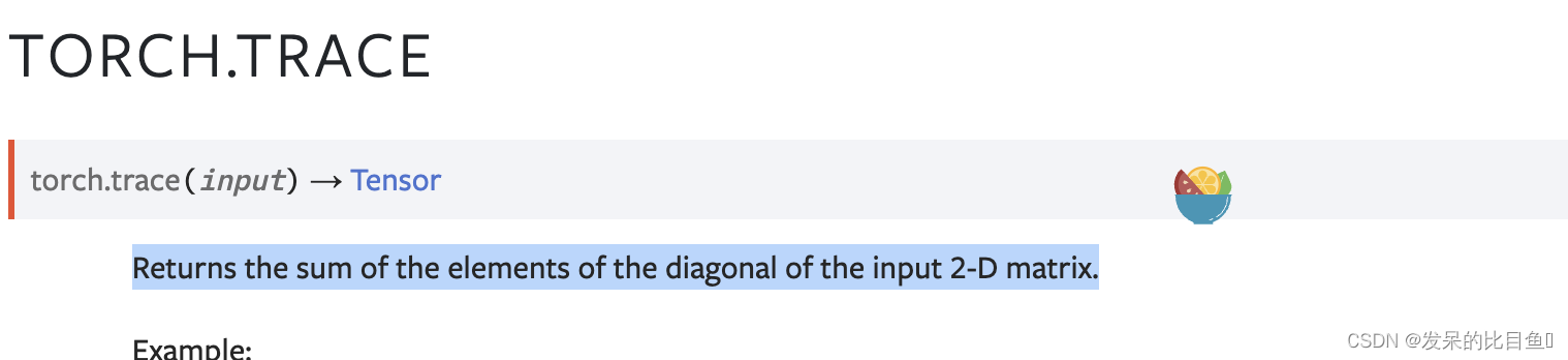
trace
返回输入二维矩阵对角线上元素的总和。
>>> x = torch.arange(1., 10.).view(3, 3)
>>> x
tensor([[ 1.,  2.,  3.],
        [ 4.,  5.,  6.],
        [ 7.,  8.,  9.]])
>>> torch.trace(x)
tensor(15.)
tril
返回矩阵的下三角部分(2-D张量)或一批矩阵输入,结果张量out的其他元素设置为0。
>>> a = torch.randn(3, 3)
>>> a
tensor([[-1.0813, -0.8619,  0.7105],
        [ 0.0935,  0.1380,  2.2112],
        [-0.3409, -0.9828,  0.0289]])
>>> torch.tril(a)
tensor([[-1.0813,  0.0000,  0.0000],
        [ 0.0935,  0.1380,  0.0000],
        [-0.3409, -0.9828,  0.0289]])

>>> b = torch.randn(4, 6)
>>> b
tensor([[ 1.2219,  0.5653, -0.2521, -0.2345,  1.2544,  0.3461],
        [ 0.4785, -0.4477,  0.6049,  0.6368,  0.8775,  0.7145],
        [ 1.1502,  3.2716, -1.1243, -0.5413,  0.3615,  0.6864],
        [-0.0614, -0.7344, -1.3164, -0.7648, -1.4024,  0.0978]])
>>> torch.tril(b, diagonal=1)
tensor([[ 1.2219,  0.5653,  0.0000,  0.0000,  0.0000,  0.0000],
        [ 0.4785, -0.4477,  0.6049,  0.0000,  0.0000,  0.0000],
        [ 1.1502,  3.2716, -1.1243, -0.5413,  0.0000,  0.0000],
        [-0.0614, -0.7344, -1.3164, -0.7648, -1.4024,  0.0000]])
>>> torch.tril(b, diagonal=-1)
tensor([[ 0.0000,  0.0000,  0.0000,  0.0000,  0.0000,  0.0000],
        [ 0.4785,  0.0000,  0.0000,  0.0000,  0.0000,  0.0000],
        [ 1.1502,  3.2716,  0.0000,  0.0000,  0.0000,  0.0000],
        [-0.0614, -0.7344, -1.3164,  0.0000,  0.0000,  0.0000]])
tril_indices
返回2-by-N张量中逐列矩阵下三角部分的索引,其中第一行包含所有索引的行坐标,第二行包含列坐标。索引是按行排序,然后按列排序。


>>> a = torch.tril_indices(3, 3)
>>> a
tensor([[0, 1, 1, 2, 2, 2],
        [0, 0, 1, 0, 1, 2]])

>>> a = torch.tril_indices(4, 3, -1)
>>> a
tensor([[1, 2, 2, 3, 3, 3],
        [0, 0, 1, 0, 1, 2]])

>>> a = torch.tril_indices(4, 3, 1)
>>> a
tensor([[0, 0, 1, 1, 1, 2, 2, 2, 3, 3, 3],
        [0, 1, 0, 1, 2, 0, 1, 2, 0, 1, 2]])
triu
返回矩阵(2-D张量)或一批矩阵的上三角部分输入,结果张量out的其他元素设置为0。

>>> a = torch.randn(3, 3)
>>> a
tensor([[ 0.2309,  0.5207,  2.0049],
        [ 0.2072, -1.0680,  0.6602],
        [ 0.3480, -0.5211, -0.4573]])
>>> torch.triu(a)
tensor([[ 0.2309,  0.5207,  2.0049],
        [ 0.0000, -1.0680,  0.6602],
        [ 0.0000,  0.0000, -0.4573]])
>>> torch.triu(a, diagonal=1)
tensor([[ 0.0000,  0.5207,  2.0049],
        [ 0.0000,  0.0000,  0.6602],
        [ 0.0000,  0.0000,  0.0000]])
>>> torch.triu(a, diagonal=-1)
tensor([[ 0.2309,  0.5207,  2.0049],
        [ 0.2072, -1.0680,  0.6602],
        [ 0.0000, -0.5211, -0.4573]])

>>> b = torch.randn(4, 6)
>>> b
tensor([[ 0.5876, -0.0794, -1.8373,  0.6654,  0.2604,  1.5235],
        [-0.2447,  0.9556, -1.2919,  1.3378, -0.1768, -1.0857],
        [ 0.4333,  0.3146,  0.6576, -1.0432,  0.9348, -0.4410],
        [-0.9888,  1.0679, -1.3337, -1.6556,  0.4798,  0.2830]])
>>> torch.triu(b, diagonal=1)
tensor([[ 0.0000, -0.0794, -1.8373,  0.6654,  0.2604,  1.5235],
        [ 0.0000,  0.0000, -1.2919,  1.3378, -0.1768, -1.0857],
        [ 0.0000,  0.0000,  0.0000, -1.0432,  0.9348, -0.4410],
        [ 0.0000,  0.0000,  0.0000,  0.0000,  0.4798,  0.2830]])
>>> torch.triu(b, diagonal=-1)
tensor([[ 0.5876, -0.0794, -1.8373,  0.6654,  0.2604,  1.5235],
        [-0.2447,  0.9556, -1.2919,  1.3378, -0.1768, -1.0857],
        [ 0.0000,  0.3146,  0.6576, -1.0432,  0.9348, -0.4410],
        [ 0.0000,  0.0000, -1.3337, -1.6556,  0.4798,  0.2830]])
triu_indices


>>> a = torch.triu_indices(3, 3)
>>> a
tensor([[0, 0, 0, 1, 1, 2],
        [0, 1, 2, 1, 2, 2]])

>>> a = torch.triu_indices(4, 3, -1)
>>> a
tensor([[0, 0, 0, 1, 1, 1, 2, 2, 3],
        [0, 1, 2, 0, 1, 2, 1, 2, 2]])

>>> a = torch.triu_indices(4, 3, 1)
>>> a
tensor([[0, 0, 1],
        [1, 2, 2]])
unflatten
将输入张量的一个维度展开到多个维度上。

>>> torch.unflatten(torch.randn(3, 4, 1), 1, (2, 2)).shape
torch.Size([3, 2, 2, 1])
>>> torch.unflatten(torch.randn(3, 4, 1), 1, (-1, 2)).shape
torch.Size([3, 2, 2, 1])
>>> torch.unflatten(torch.randn(5, 12, 3), -1, (2, 2, 3, 1, 1)).shape
torch.Size([5, 2, 2, 3, 1, 1, 3])
vander
生成范德蒙德矩阵。

>>> x = torch.tensor([1, 2, 3, 5])
>>> torch.vander(x)
tensor([[  1,   1,   1,   1],
        [  8,   4,   2,   1],
        [ 27,   9,   3,   1],
        [125,  25,   5,   1]])
>>> torch.vander(x, N=3)
tensor([[ 1,  1,  1],
        [ 4,  2,  1],
        [ 9,  3,  1],
        [25,  5,  1]])
>>> torch.vander(x, N=3, increasing=True)
tensor([[ 1,  1,  1],
        [ 1,  2,  4],
        [ 1,  3,  9],
        [ 1,  5, 25]])
view_as_real
返回作为实数张量的输入视图。对于大小为m1,m2,…,mi的输入复张量,此函数返回大小为m1、m2,…、mi,2的新实张量,其中大小为2的最后一个维度表示复数的实分量和虚分量

>>> x=torch.randn(4, dtype=torch.cfloat)
>>> x
tensor([(0.4737-0.3839j), (-0.2098-0.6699j), (0.3470-0.9451j), (-0.5174-1.3136j)])
>>> torch.view_as_real(x)
tensor([[ 0.4737, -0.3839],
        [-0.2098, -0.6699],
        [ 0.3470, -0.9451],
        [-0.5174, -1.3136]])
view_as_complex
返回作为复数张量的输入视图。对于大小为m1,m2,…,mi,2的输入复张量,此函数返回大小为m1、m2,…、mi的新复张量,其中输入张量的最后一个维度预计表示复数的实分量和虚分量。

>>> x=torch.randn(4, 2)
>>> x
tensor([[ 1.6116, -0.5772],
        [-1.4606, -0.9120],
        [ 0.0786, -1.7497],
        [-0.6561, -1.6623]])
>>> torch.view_as_complex(x)
tensor([(1.6116-0.5772j), (-1.4606-0.9120j), (0.0786-1.7497j), (-0.6561-1.6623j)])
resolve_conj
如果输入的共轭位设置为True,则返回具有物化共轭的新张量,否则返回输入。输出张量的共轭位将始终设置为False。

>>> x = torch.tensor([-1 + 1j, -2 + 2j, 3 - 3j])
>>> y = x.conj()
>>> y.is_conj()
True
>>> z = y.resolve_conj()
>>> z
tensor([-1 - 1j, -2 - 2j, 3 + 3j])
>>> z.is_conj()
False
resolve_neg
如果输入的负位设置为True,则返回具有物化否定的新张量,否则返回输入。输出张量的负位将始终设置为False。:param input:输入张量。:类型输入:Tensor

>>> x = torch.tensor([-1 + 1j, -2 + 2j, 3 - 3j])
>>> y = x.conj()
>>> z = y.imag
>>> z.is_neg()
True
>>> out = y.resolve_neg()
>>> out
tensor([-1, -2, -3])
>>> out.is_neg()
False


 908
908


 被折叠的 条评论
为什么被折叠?
被折叠的 条评论
为什么被折叠?
 到【灌水乐园】发言


