Boundary Conditions Theory

Every model requires an appropriate set of boundary conditions to represent the system’s relationship with the surrounding systems. In the case of a groundwater flow model, boundary conditions will describe the exchange of flow between the model and the external system. In the case of a mass transport model, the boundary conditions will also describe the exchange of solute mass between the model and the external system.

The following sections present an overview of the boundary condition packages supported in Visual MODFLOW Flex. Each section includes a brief description of the boundary condition, including the input data required by MODFLOW and the supported data objects for defining the boundary condition geometry. The following boundary conditions are discussed in this section:

•Well

oWells (WEL)

oMulti-Node Wells (MNW1/MNW2)

•Constant Head (CHD)

•River (RIV)

•General Head (GHD)

•Drain (DRN)

•Streamflow-Routing (SFR2)

•Recharge (RCH)

•Evaporation (EVT)

•Lake (LAK)

•Specified Flux (FHB)

•Time-varying Material Properties (TMP)

•Unsaturated Zone Flow (UZF)

•Mass Source Loading (SRC)

Well

There are several different types of Well boundary condition supported in Visual MODFLOW Flex that each include different conceptualizations of groundwater withdrawals/injections via wells via distinct boundary condition packages:

Well Types

Well Model	WEL	MNW1	MNW2
Engines
MF-2000
MF-2005
MF-NWT
MF-LGR
SEAWAT
MF-SURFACT
MF-USG

WEL Package

The well (WEL) package is the simplest boundary condition used to simulate wells in MODFLOW.  In the WEL package, wells (and other features) are conceptualized as points sinks that withdraw water from or sources that add water to the model at a constant rate during a stress period, where the rate is independent of both the cell area and head in the cell.

The MODFLOW input data for Well cells is stored in the projectname.WEL file. You can define the location for vertical or non-vertical wells (which include the well path and the screen location). When you translate your conceptual model to MODFLOW format, the well screen locations are converted to set of pumping well cells.  Another option is to define a specified flux or drain boundary condition in Visual MODFLOW Flex.

Conceptualization in MODFLOW

Visual MODFLOW Flex supports pumping wells with one or more screen intervals along the path of the well bore, including well screens that partially penetrate a model layer. However, it is important to note that the WEL package in MODFLOW does not include any special considerations for multiple well screens or grid cells containing partially penetrating well screens. MODFLOW treats WEL pumping wells as simple flux boundary conditions, such that each grid cell intersecting a well screen is assigned a specified flux that is constant for a given stress period. In a situation where a well is screened across several model layers, Visual MODFLOW Flex uses the length of the well screen intersecting each model layer to determine the proportion of the total well pumping rate assigned to each well grid cell in the model, even though MODFLOW considers a cell to be screened over its entire vertical length, regardless of the length of screen assigned to the cell. The following equation is used to calculate the pumping rate for each grid cell:

        (1)

where:

 is the specified discharge from the ith cell to a particular well in a given stress period        [L3/T]

 is the total specified pumping rate for all screens in a particular well in a given stress period        [L3/T]

 is the screen length of screen in the ith cell        [L]

 is the hydraulic conductivity in the x-direction in the ith cell        [L/T]

 represents the sum of the products of screen length and hydraulic conductivities in the x-direction of all cell penetrated by the well.        [L2/T]

The WEL package approach, in which a well screened over one or more cells/layers is represented as a set of independent specified flow rates, fails to take into account the inter-connection between various layers provided by the well. One of the most significant problems related to this approach is that MODLFLOW will inactivate cells and their boundary conditions when the water table drops below the bottom of the grid cell (i.e. when the grid cell becomes dry). This automatically reduces the total pumping rate of the well, and may cause the water table to “rebound” and re-activate the well grid cell. This type of on-again-off-again behavior for the pumping well(s) causes the solution to oscillate, and may prevent the model from converging to a solution. In the event the model does converge to a solution, the model results may be misleading if one or more pumping wells have lower than expected total pumping rates.

Alternately, a multi-layer well can sometimes be simulated by means of a vertical column of high permeability cells with a screen at the bottom of the column. In this case, if the top part of the model becomes dry, the total pumping rate is unaffected. This also takes into account the vertical inter-connection between layers. The downside of this approach is that the conductivity contrasts can lead to convergence problems.

The MNW1 and MNW2 packages (described below) provide better representation of wells screened over multiple layers. Both of these packages are able to dynamically redistribute pumping rates to the remaining active grid cells if one or more cells in the screened interval goes dry, thereby more accurately simulating the real-world effects of partial overpumping of a well screened over multiple layers.

Despite the limitations described above, the WEL package includes some advantages over the MNW packages described below, including that it has minimal input data requirements and it is very computationally efficient and stable.

Required Data

In Visual MODFLOW Flex, pumping well boundary conditions in the WEL package are defined using the well data contained in a wells data object. During the boundary condition creation process, you will be required to select a wells data object from the Data Explorer.

A well can only be used if it meets the following requirements:

•The pumping well must be located within the simulation domain

•One or more screens must be defined for the pumping well

•A pumping schedule with at least one stress period must be defined for the pumping well

For information on importing well data, please see "Importing Wells" section. For information on defining well data for existing wells data objects, please see the "Well Table" section

MNW1 and MNW2 Packages

Pumpage from aquifer systems is commonly more complex than the simple considerations included in the WEL package described above. The Multi-Node Well packages (MNW1 and MNW2) were developed to include additional complexities associated with well screens that span multiple layers/cells, including:

•the head in the well is distinct from the head(s) in the neighboring formation,

•pumping is from the entire well, and

•pumping rates may be constrained by the physical limitations of the pump configuration

For example, heads in aquifers that surround a well are likely to vary along the length of a screen, particularly if the well screen penetrates multiple aquifers or has a long horizontal extent. When pumping, recharge, or no user-specified inflow or outflow occurs in wells that are screened across multiple aquifers or in a single aquifer, there can be significant hydraulic effects on the ground-water flow system. The Multi-Node Well packages (MNW1 and MNW2) have been integrated in Visual MODFLOW Flex to help simulate intraborehole flow occurring in wells with screens that span multiple layers.  MNW1 was the original implementation by the USGS (Halford and Hanson, 2002) and provided a great deal of flexibility for specifying well input parameters that may change over time.  MNW2 provides a somewhat streamlined input structure (Konikow, et al., 2009) and allows for some additional well configurations/processes, most notably those associated with non-vertical wells.

Conceptualization in MODFLOW

Visual MODFLOW Flex supports pumping wells with one or more screen intervals along the path of the well bore, including well screens that partially penetrate a model layer. In the Multi-Node Well packages, the flow rate from the pumping well and heads in the well and adjacent model cells are based on an analogous approximation of resistors in a network:

Source: Halford and Hanson (2002)

        (2)

where:

 is the total flow rate from the well (positive for injection and negative for withdrawal) [L3/T]

 is the head in the well [L],

 is the head in the formation at model cell i along the well screen(s) [L],

 is the cell-to-well conductance at model cell i along the well screen(s) [L2/T]

The cell-to-well conductance in the MNW package is based on the following equations (Halford and Hanson, 2002 and Konikow, et al, 2009):

        (3)

where:

 is the linear formation head-loss coefficient given by [T/L2]:

        (4)

 is the linear well head-loss coefficient given by [T/L2]:

        (5)

 is the non-linear well head-loss coefficient

 is the non-linear well head-loss exponent (1.0 - 3.5, usually 2.0) [L2/T]

 is thickness of the formation in model cell i [L]

 is the effective radius of the rectilinear finite difference cell which is calculated automatically by Visual MODFLOW Flex using equation 6 in Halford and Hanson (2002) [L]

 is the radius of the well screen [L]

 is a Skin factor for model cell i, based on the following equation [-]:

        (6)

 is the hydraulic conductivity of the formation in the x-direction in the ith cell [L/T],

 is the hydraulic conductivity in the formation in the y-direction in the ith cell [L/T],

 is the hydraulic conductivity of the well skin along the borehole [L/T],

 is length of the well screen in model cell i [L]

 is the radius of the well skin [L],

For more information on the development and theory behind these packages, please see the original USGS reports for MNW1 by Halford and Hanson, (2002) and for MNW2 by Konikow, et al., (2009).

Required Data

In Visual MODFLOW Flex, pumping well boundary conditions are defined using the well data contained in a wells data object. During the boundary condition creation process, you will be required to select an existing wells data object from the Data Explorer or create a new one.

Multi-node wells must include the following minimum information:

•The pumping well must be located within the simulation domain

•One or more screens must be defined for the pumping well

•A pumping schedule with at least one stress period must be defined for the pumping well

•Parameters for well hydraulics

Well Loss parameters

There are several options in the multi-node well packages to define the head loss between the well and the adjacent cells in each of the multi-node well packages.  The options and their relevant input variables are presented in the Table 1 and Table 2 below for the MNW1 and MNW2 packages, respectively, while descriptions of the relevant input variables are presented further below.

Table 1. Supported MNW1 loss types in Visual MODFLOW Flex

Loss Model*	MNW1 Option*	Required Input Properties
		Rw **	Rskin **	KSkin **	B **	C **	P *	CWC **	CWCDist **
None	Skin	0
Thiem	Skin		Rw
Skin	Skin
Linear	Linear
Non-Linear	Non-Linear
Specify CWC	Skin	-CWC

Notes: * the property is global and specified once for all wells in the MNW1 package ** the property is transient and specified for each well/stress period. Flex will distribute values each to cell intersecting the well screen(s)

Table 2. Supported MNW2 loss types in Visual MODFLOW Flex

Loss Model*	MNW2 Option*	Required Input Properties
		Rw **	Rskin **	KSkin **	B **	C **	P *	CWC **	CWCDist **
None	None
Thiem	Thiem
Skin	Skin
Linear	General					0
Non-Linear	General
Specify CWC	SpecifyCWC

Notes: * the property is static and specified once for each well ** the property is static and specified once for each well. Flex will distribute values to each cell intersecting the well screen(s)

The input variables for the well loss models are as follows:

•Rw: Radius of the well screen (L)

•RSkin: Radius of the well skin (L)

•KSkin: Hydraulic conductivity of the well skin (L/T)

•B: Linear well loss coefficient

•C: Non-linear well loss coefficient

•P: Non-linear well loss exponent (1.0 to 3.5, default 2.0)

•CWC: cell to well loss coefficient

•CWC Dist: Option for defining how the CWC coefficient is distributed across the cell(s) spanning the screen:

oBy Cell,

oBy Screen Cell Thickness,

oBy Screen Cell Transmissivity

Well Performance and Constraints

The multi-node well packages provide input variables that allow you to define conditions on pumping in the well.

Input Parameter	MNW1*	MNW2**
Water Limit
HLim
Href
QCut
Qfrcmn
Qfrcmx

Notes: * input variables are transient are specified for each well in each stress period. Flex will distribute values to cell intersecting the well screen(s) ** the property is static and specified once for each well

The input variables for the well performance and constraints are as follows:

•WaterLimit: Option to set the reference type for HLim and Href

o"Water Level": water level constraints are based on the absolute water level in the specified well

o"Drawdown": water level contraints are based on relative water level in the specified well (drawdown)

•HLim: limiting water level in the well (a minimum for discharging wells [Q<0] and a maximum for injection wells [Q>0]. For example, if the head in the well falls below this value in a discharging well, then pumping in the well ceases.

•Href: Reference elevation for the limiting water level (HLIM). If the value of HREF is greater than the maximum water level at the beginning of stress period 1, HREF is set to the simulated water level at the location of the head/drawdown-limited well.

•QCut: Option to set pumping rate limit types for Qfrcmn and Qfrcmx, either by absolute rate or by percent

oQfrcmn: Pumping rate or fraction (see QCUT) below which pumping will cease

oQfrcmx: Pumping rate or fraction (see QCUT) above which pumping will resume/be reactivated

Supported Geometry

Wells in Visual MODFLOW Flex are based on well data objects. For information on importing well data, please see "Importing Wells" section.

For information on defining well data for existing wells data objects, please see the "Well Table" section.

Constant Head

The Specified Head boundary condition, also known as Constant Head in VMOD Flex, is used to fix the head value in selected grid cells regardless of the system conditions in the surrounding grid cells, thus acting as a potentially infinite source of water entering the system, or as an infinite sink for water leaving the system. Therefore, specified head boundary conditions can have a significant influence on the results of a simulation, and may lead to unrealistic predictions, particularly when used in locations close to the area of interest.

During translation, VMOD Flex uses the Time-Variant Specified-Head (CHD) Package provided with MODFLOW. The MODFLOW input data for Specified Head cells is stored in projectname.CHD file.

Unlike most other transient MODFLOW boundary condition packages, the Constant-Head package allows the specified heads to be linearly interpolated in time between the beginning and end of each stress period, such that the specified head for a grid cell may change at each time step within a given stress period.  If the simulation is steady-state, the specified starting head value will be used from the first stress period. Note, this is no longer the case, in MODFLOW-6 which only supports single values for each stress period using the basic input method.

Required Data

The Specified-Head package requires the following information for each specified head grid cell for each stress period:

•Start Head: Specified head value at the beginning of the stress period

•Stop Head: Specified head value at the end of the stress period

Supported Geometry

The geometry for Specified Head boundary conditions can be specified using Polylines or Polygons

A Note on Leakance vs. Conductance

Some Type-3 (Head-Dependent Flux) boundary conditions (e.g. river and general head) require defining a conductance parameter (for MODFLOW).  Conductance is a  numerical parameter representing the resistance to flow between the cell assigned with that boundary condition and the surrounding cells. Conductance between cells is calculated using some average hydraulic conductivity of the cells, the area of the interface between the cells and the distance between the cell centers. The Conductance calculation requires the cell geometry (cell interfaces). In Visual MODFLOW Flex, when you create a new conceptual boundary condition, this is done using shapes: polyline, polygon, and side faces. At this point, there is no notion of cell geometry, as a result, the conductance cannot be calculated since the cell face area cannot yet be calculated.  For this reason, you are asked to define "Leakance" instead of "Conductance".  Leakance is a conceptual (hydrogeologic) term, and is expressed per unit area (if the conceptual boundary condition object is a polygon) or per unit length (if the conceptual boundary condition object is a polyline). When you create the boundary condition, the Leakance can be calculated based on other defined parameters, or it can be explicitly defined. When you look at the numerical representation (cell realization) of the boundary condition, you will see "Conductance" as the parameter, since this value can be calculated based on the intersecting cell geometry.  For a boundary condition assigned with a polygon or side face, the Leakance is multiplied by the cell area, in order to get Conductance.  For a boundary condition assigned with a polyline, the Leakance is multiplied by the length of the line that intersects the cell, in order to get the Conductance. More details on this can be found at: Introduction.

River

The MODFLOW River Package simulates surface water/groundwater interaction via a seepage layer separating the surface water body from the groundwater system. VMOD Flex uses the River Package included in MODFLOW. MODFLOW input data for River grid cells is stored in projectname.RIV file.

Conceptualization in MODFLOW

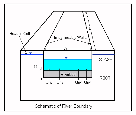
The River boundary condition is a simple conceptualization of surface water features used to simulate the influence of a surface water body on the groundwater flow system. Surface water bodies such as rivers, streams, lakes and swamps may either contribute water to the groundwater system, or act as groundwater discharge zones, depending on the hydraulic gradient between the surface water body and the groundwater system.  The conceptualization of rivers (or other surface water features that this boundary condition is used to represent) is represented as a seepage layer of bed sediments that is assumed to be a flat bottom, with no seepage through the sides of the channel as shown below:

The RIV package approach, fails to take into account the mass balance in the overlying surface water feature and can supply or remove an infinite amount of water to/from the groundwater system. The can produce non-physical results with unexpected amounts of water being exchanged between the groundwater and surface water system both locally and regionally in the model.

The Streamflow-Routing (SFR) package (described below) provides a better representation of river systems, and includes conceptualizations of flow within and between stream reaches, which are entirely ignored in the RIV conceptualization

Required Data

The MODFLOW River Package input file requires the following information for each grid cell containing a River boundary;

•River Stage: The free water surface elevation of the surface water body. This elevation may change with time.

•Riverbed Bottom: The elevation of the bottom of the seepage layer (bedding material) of the surface water body.

•Conductance: A numerical parameter representing the resistance to flow between the surface water body and the groundwater caused by the seepage layer (riverbed).

The Conductance value (C) may be calculated from the length of a reach (L) through a cell, the width of the river (W) in the cell, the thickness of the riverbed (M), and the vertical hydraulic conductivity of the riverbed material (K) using the following formula:

        (7)

For situations where the River package is used to simulate lakes or wetlands, the L and W variables would correspond to the X-Y dimension of the River boundary grid cells. When a River boundary condition is assigned, the Use default Leakance option is automatically selected.

If the Use default Leakance option is selected, the River boundary condition requires the following data:

•River Stage: The free water surface elevation of the surface water body. [L]

•Riverbed Bottom: The elevation of the bottom of the seepage layer (bedding material) of the surface water body.  [L]

•Riverbed Thickness: Thickness of the riverbed (seepage layer) [L].

•Leakance: A numerical parameter representing the resistance to flow between the surface water body and the aquifer (this field is read-only and is calculated using the formula described below). [L2/T or L/T, see below]

•Riverbed Kz: Vertical hydraulic conductivity of the riverbed material. [L/T]

•River Width: Width of the river. [L]

When a polyline is used to define the river geometry, the default conductance formula is as follows:

        (8)

When a polygon is used to define the river geometry, the default conductance formula is as follows:

        (9)

where:

$COND: is the Conductance

$RCHLNG: is the reach length of the river line in each grid cell

$WIDTH: is the River Width in each grid cell

$K: is the Riverbed Kz

$UCTOCOND: is the conversion factor for converting the $K value to the same L and T units used by $COND. $UCTOCOND is automatically calculated by Visual MODFLOW Flex.

$RBTHICK: is the Riverbed Thickness

$DX: is the length of each grid cell in the X-direction

$DY: is the length of each grid cell in the Y-direction

If the "Use default Leakance" option is turned off, the fields used for calculating the River Leakance value (Riverbed Thickness, Riverbed Kz, and River Width) are removed from the table, and the Leakance field becomes a writable field where a value may be entered.

Supported Geometry

The geometry for River boundary conditions can be specified using polylines or polygons

General Head

VMOD Flex supports translation of the General-Head Boundary Package included with MODFLOW. The MODFLOW input data for General-Head grid cells is stored in the projectname.GHB file.

Conceptualization in MODFLOW

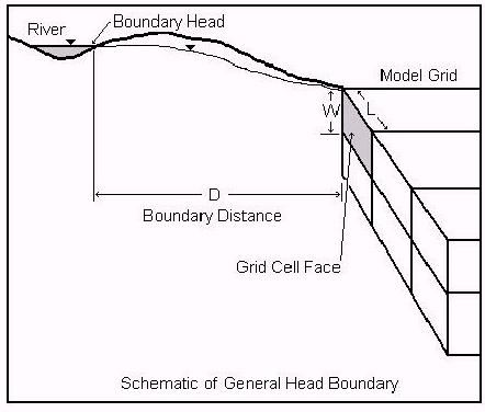
The function of the General-Head Boundary (GHB) Package is mathematically similar to that of the River, Drain, and Evapotranspiration Packages. Flow into or out of a cell from an external source is provided in proportion to the difference between the head in the cell and the reference head assigned to the external source. The application of this boundary condition is intended to be general, as indicated by its name, but the typical application of this boundary condition is to represent heads in a model that are influenced by a large surface water body outside the model domain with a known water elevation. The purpose of using this boundary condition is to avoid unnecessarily extending the model domain outward to meet the element influencing the head in the model. As a result, the General Head boundary condition is usually assigned along the outside edges (sides) of the simulation model domain. This scenario is illustrated in the following figure.

The primary differences between the General-Head boundary and the Specified Head boundary are:

•the model solves for the head values in the General-Head grid cells whereas the head values are specified in Constant Head cells.

•the General-Head grid cells do not act as infinite sources of water whereas Specified Head cells can provide an infinite amount of water as required to maintain the specified head. Therefore, under some circumstances, the General-Head grid cells may become dry cells.

Required Data

The General-Head Boundary Package requires the following information for each General-Head grid cell:

•Stage: This is the head of the external source/sink. This head may be physically based, such as a large lake, or may be obtained through model calibration.

•Conductance: The is a numerical parameter that represents the resistance to flow between the boundary head and the model domain.

In contrast to the River, Drain, and Evapotranspiration packages, the General Head package provides no limiting value of head to bind the linear function in either direction. Therefore, as the head difference between a model cell and the boundary head increases/decreases, flow into or out of the cell continues to increase without limit. Accordingly, care must be used to ensure that unrealistic flows into or out of the system do not develop during the simulation.

The leakance value may be physically based, representing the conductance associated with an aquifer between the model area and a large lake, or may be obtained through model calibration. The leakance value (C) for the scenarios illustrated in the preceding figure may be calculated using the following formula:

        (10)

where:

 is the surface area of the grid cell face exchanging flow with the external source/sink

 is the average hydraulic conductivity of the aquifer material separating the external source/sink from the model grid

 is the distance from the external source/sink to the model grid

When a General-Head boundary condition is assigned, the Use default leakance option is automatically selected.

If the "Use default leakance" option is selected, the General-Head boundary condition requires the following data:

•Stage: The head value for the external source/sink

•Leakance: A numerical parameter representing the resistance to flow between the boundary head and the model domain (this field is read-only and is calculated using formula described below)

•Distance to Reservoir: The distance from the external source/sink to the General-Head grid cell

•General Head Average Conductivity: The average hydraulic conductivity of the aquifer material separating the external source/sink from the model grid

The default formula used to calculate the Leakance value for the General-Head boundary is:

        (11)

where:

$COND: is the Leakance for each General-Head grid cell

$KAVG: is the Average Conductivity

$FACEAREA: is the surface area of the selected grid cell Face for each General-Head grid cell (automatically calculated during translation)

$UCTOCOND: is the conversion factor for converting the $K value to the same Length (L) and Time (T) units used by $COND. $UCTOCOND is automatically calculated by Visual MODFLOW Flex.

$DIST: is the Boundary Distance, the distance from the external source to the assigned general head boundary

If the "Use default conductance" formula option is not selected, the fields used for calculating the General-Head Conductance value (Distance to Reservoir, Average Conductivity) are removed from the table, and the Leakance field becomes a writable field where a value may be entered.

Supported Geometry

The geometry for General-Head boundary conditions can be specified using a polygon data objects.

Drain

VMOD Flex supports the standard Drain Boundary Package included with MODFLOW. The MODFLOW input data for Drain grid cells is stored in the projectname.DRN file. Currently, for finite element model translation, this boundary condition is not supported.

The Drain Package in MODFLOW is designed to simulate the effects of features such as agricultural drains, which remove water from the aquifer at a rate proportional to the difference between the head in the aquifer and some fixed head or elevation. The Drain package assumes the drain has no effect if the head in the aquifer falls below the fixed head of the drain.

VMOD Flex支持MODFLOW中包含的标准排水边界包。排水格单元的MODFLOW输入数据存储在projectname.DRN文件中。目前，对于有限元模型的转换，此边界条件尚不受支持。

MODFLOW中的排水包设计用于模拟诸如农业排水等特征的效应，这些特征以水力头在含水层中的差异与某个固定水头或高程成比例地移除水。排水包假设如果含水层中的水头低于排水口的固定水头，则排水口不会产生任何影响。

Required Data

The Drain Package requires the following information as input for each cell containing this boundary condition:

•Elevation: The drain elevation, or drain head of the free surface of water within the drain. The drain is assumed to run only partially full, so that the head within the drain is approximately equal to the median elevation of the drain.

•Leakance: The drain leakance is a lumped coefficient describing the head loss between the drain and the groundwater system. This loss is caused by converging flow patterns near the drain, the presence of foreign material around the drain, channel bed materials, the drain wall, and the degree to which the drain pipe openings may be blocked by chemical precipitates, plant roots, etc.

There is no general formulation for calculating drain leakance. In most situations, the detailed information required to calculate drain leakance is not available to the groundwater modeler. These details include the detailed head distribution around the drain, aquifer hydraulic conductivity near the drain, distribution of fill material, number and size of the drain pipe openings, the amount of clogging materials, and the hydraulic conductivity of clogging materials. It is common to calculate drain leakance from measured values of flow rate and head difference. Drain leakance value is usually adjusted during model calibration.

排水包需要以下信息作为每个包含该边界条件的单元格的输入：

• 高程：排水高程，或者排水内部自由水面的排水头。假定排水仅部分充满，因此排水内的头部大约等于排水的中位高程。

• 渗漏系数：排水渗漏系数是描述排水和地下水系统之间压力损失的总系数。这种损失是由排水附近的汇流流型、排水周围的异物、河道床材料、排水壁和排水管开口可能被化学沉淀物、植物根等阻塞程度引起的。

没有用于计算排水渗漏系数的通用公式。在大多数情况下，用于计算排水渗漏系数所需的详细信息并不为地下水模型制作者所掌握。这些细节包括排水周围的详细头部分布、排水附近的含水层水力传导率、填料分布、排水管开口的数量和大小、阻塞材料的量以及阻塞材料的水力传导率。通常，排水渗漏系数是从流量和压力差的测量值中计算出来的。在模型校准期间通常会调整排水渗漏系数的值。

When a polyline is used to define the boundary condition geometry, the default formula for the leakance is as follows:

当使用折线来定义边界条件几何形状时，泄漏率的默认公式如下：

        (11)

When a polygon is used to define the boundary condition geometry, the default leakance formula is as follows:

当多边形被用来定义边界条件几何形状时，默认的渗透性公式如下：

        (12)

where:

$COND: is the Leakance for each drain cell

$RCHLNG: is the reach length of the drain in each grid cell

$LCOND: is the Leakance per unit length of the drain in each grid cell

$SCOND: is the Leakance per unit area of the drain in each grid cell

$DX: is the length of each grid cell in the X-direction

$DY: is the length of each grid cell in the Y-direction

If the Use default leakance option is turned off, the fields used for calculating the Drain Leakance value (Leakance per unit length or area) are removed from the table and the Leakance field becomes a read/write field where any value may be entered.

$COND：每个排水单元的渗漏率

$RCHLNG：每个网格单元中排水的长度

$LCOND：每个网格单元中排水的单位长度渗漏率

$SCOND：每个网格单元中排水的单位面积渗漏率

$DX：X方向上每个网格单元的长度

$DY：Y方向上每个网格单元的长度 如果关闭默认渗漏率选项，则用于计算排水渗漏率值（单位长度或面积的渗漏率）的字段将从表中删除，渗漏率字段将变成读/写字段，可以输入任何值。

Supported Geometry

The geometry for General-Head boundary conditions can be specified using polygon or polylines

Streamflow-Routing (SFR2)

Flow in surface water systems is commonly more complex than the simple considerations included in the head-dependent flux boundaries such as RIV, DRN, and GHB packages described above. The streamflow-routing (SFR2) package was developed to include additional/optional complexities associated with surface water features, including:

•mass balance (including optional flow routing) between stream reaches,

•estimation of flow/water depth in stream reaches, and

•unsaturated flow to groundwater system from perched streams

For more information, see the USGS documentation for SFR1 (Prudic et. al., 2004) and SFR2 (Niswonger and Prudic, 2005).  The online documentation for SFR2 contains additional information that supplements the USGS documentation, including documentation of the minor differences between the input structures for the versions of MODFLOW (e.g. -2000, -2005, -NWT, -LGR).

 Please note: SFR2 is not currently supported with MODFLOW-USG, MODFLOW-6, MODFLOW-SURFACT, or SEAWAT in Visual MODFLOW Flex.

Conceptualization in MODFLOW

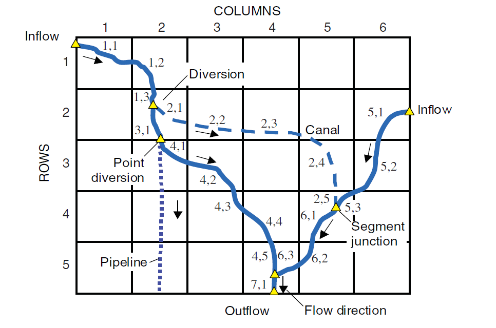
Visual MODFLOW Flex supports surface water drainage systems as one or more networks of directed linear stream segments that may also be connected to polygonal lakes. Each segment or lake is an indexed single part polyline or polygon, respectively. The indices of each stream segment must ascend in the downstream direction and points of confluence (junctions) may either have multiple upstream connections to a single downstream segment (many to one) or one upstream connection to one or more downstream segments (one to many), but not multiple upstream connections to multiple downstream connections (many to many) as this configuration would lead to ambiguous flow routing given the algorithms implemented in SFR2.

Example Stream Network: streams are denoted by segment,reach. Where a segment is the polyline in the network and a reach is the portion of a segment within a given cell.  Segment and reach indices must increase in the downstream direction. Source: Prudic, et. al. (2004)

Mass Balance in Streams

Stream flows are estimated in the SFR2 package by a local and global mass balance on stream reaches within the network:

        (13)

        (14)

where:

 is the total inflow to a stream reach [L3/T]

 is the total outflow from a stream reach [L3/T]

 is a specified inflow to the first reach in a segment [L3/T]. For segments originating within the model domain, this value is zero and non-zero for segments at the model boundary with upstream flows from outside the lateral extents of the model,

 is the estimated outflow from each upstream tributary [L3/T],

 is the direct runoff from overland flow into the reach [L3/T],

 is the direct precipitation into the stream reach [L3/T],

 is the groundwater leakage from the stream reach to the hydraulically connected aquifer[L3/T]

 is the estimated outflow from the reach [L3/T],

 is an optionally specified diversion from the reach [L3/T],

 is the direct evapotranspiration from the reach [L3/T],

 is the groundwater leakage from a perched stream reach to an underlying aquifer through the vadose zone [L3/T]

In order to estimate groundwater leakage from the stream (whether hydraulically connected or perched), the SFR2 package estimates the depth of the stream at the midpoint of each reach to obtain a head value by adding the estimated depth (dri) at the midpoint of the reach to the estimated bottom elevation of each reach (zri). The bottom elevation at the midpoint is estimated by linearly interpolating the stream bottom elevations specified at the upstream and downstream ends of each segment.

Streamflow Diversions

In general, the stream network in the SFR2 package is assumed to bifurcate in the upstream direction only and the network always converges in the downstream direction towards a single watershed outlet.  However, in some cases, flows in the downstream may diverge, either due to natural features (e.g. braided channels, sandbars, etc.) or constructed features (e.g. water intakes, irrigation ditches, canals, etc.).  In the former case, where flow always converges, calculating the inflows to the downstream segment is trivial in that they are the sum of the outflows from the upstream segments.  However, in the case where flows diverge in the downstream direction, the amount of flow must be divided up to each downstream segment.  The SFR2 package provides four options:

•Reduce to available (IPRIOR=0): all available flow at the end of the last reach of a segment up to the rate specified will be diverted from the segment. Thus, if flow in the stream is less than the specified diversion, all available flow in the stream will be diverted, and none will remain in the channel. This option is common to many diversions in the western United States and is the default option for diversions.

•Reduce to None (IPRIOR=1): the specified diversion will only occur if flow in the stream is greater than that of the diversion, if flow is less than the specified diversion, then no flow is diverted and all flow remains in the channel.

•Fraction of Available (IPRIOR=2): a specified fraction of the available flow will be diverted

•Divert Excess (IPRIOR=3): all flow in excess of a specified rate will be diverted. This option is typically used for flood control in which all excess flow is diverted away from the main channel during peak discharge.

Water entering a diversion is subtracted from the end of the last reach of a segment; any remaining flow at the end of the last reach of a segment is added as tributary inflow at the beginning of the first reach in the next downstream segment.

Stream Depth

The depth of the stream in each reach is estimated using one of two supported options in Visual MODFLOW Flex:

•Specified Depth (ICalc=0): the stream depth will be specified at both the upstream and downstream end of the segment and linearly interpolated to the midpoint of each reach

•Variable depth (ICalc=1): the stream depth will be estimated based on the estimated discharge at the midpoint of the stream and Manning's equation, as described below.

The estimated discharge at the midpoint of a reach is based on the assumption that the distributed inflows and outflows are uniform along the length of the channel, that point inflows are located at the upstream end of the reach, and that point outflows occur at the downstream end of the reach and are ignored as follows:

        (15)        

The depth of the stream at the midpoint is estimated based on a rearranged form of the Manning equation for a "wide" rectangular channel (e.g. the stream is much wider than the depth of the stream and the hydraulic radius is approximately equal to the width of the stream):

        (16)

where:

 is the estimated stream depth at the midpoint of the reach [L3/T],

 is the Manning roughness parameter [-],

 is a dimensional constant, which is 1.0 for flow units in m3/s and 1.486 for units of ft3/s [L1/3/T],

 is the width of the stream [-],

 is the slope of the reach which is estimated by Flex as from the segment length and its upstream and downstream elevations

In the case of variable stream depths calculated by the SFR2 package, the depth of the stream is both an input to the estimate of the groundwater leakance and is indirectly derived from it, which creates a circular dependence that is resolved using Newton-Raphson iterations and a specified tolerance as discussed in Prudic et al (2004).

Stream Leakance (Saturated)

In the case where the stream is directly connected to the groundwater system (i.e. the water table is above the bottom of the stream bed, stream leakance is calculated using the Darcy's law, similar to the implementation in the RIV package:

        (17)

where:

 is (plan view) area of the streambed in the reach [L2],

 is hydraulic conductivity of the bed sediments [L/T],

 is the thickness of the bed sediments [L],

 is the head in the stream reach [L],

 is the head in the groundwater system in the shared model cell [L].

In this case, the exchange between the groundwater system and the stream will be considered to occur instantaneously within the current time step.

Stream Leakance (Unsaturated)

The SFR2 package can also optionally include stream leakance through the unsaturated zone where stream reaches are perched (i.e. in cases where the calculated groundwater head in a cell falls below the bottom of the stream bed). In such reaches, the stream will discharge via the unsaturated zone using the same approach as implemented in the UZF package except:

        (18)

where:

 is the elevation of the stream bed [L]

Assumptions and Limitations

Major assumptions inherent in the SFR2 approach include the following:

•streamflow is one-dimensional and in the direction of the channel segments

•when the channel depth is specified as variable:

osteady flow in the channel is assumed unless flow routing is active (i.e. TRANSROUTE is specified and IRTFLG=1), in which case the kinematic wave equation is used and dynamic wave effects are ignored

ostream channels are sufficiently wide relative to stream depth such that the hydraulic radius is adequately described by the width of the stream in Manning's equation

oa single value of Manning's roughness coefficient is adequate to estimate stream depths for the range of simulated discharges in each segment (e.g. the stream does not oscillate between flowing within the channel banks and spilling into the floodplain with a significantly different roughness)

ono backwater effects are considered

•flows are routed to downstream reaches based on continuity and the SFR package is not recommended for modeling the surface water flows, depths, or the transient exchange of water between stream reaches and the groundwater system for evaluations of short-term (seconds to days) effects.  The inclusion of the kinematic wave routing (i.e. TRANSROUTE option and IRTFLG=1) may provide some improvements as described in Markstrom, et al. (2008).

Other assumptions are also inherent in the implementation of SFR2, a more comprehensive complete list of the assumptions is included in the documentation references discussed above which should be consulted as part of the model development process.

Required Parameters

In Visual MODFLOW Flex, the SFR2 Package requires a more complex set of inputs than the other boundary conditions and as such is defined in its own workflow. Surface Water inputs are grid independent and are based on a set of parameterized vector geometries that define the surface water network consisting of connected/directed stream segments and optional lake polygons. Inputs for each of these is defined in the Surface Water Network Data section.

Supported Geometry

Surface Water inputs are grid-independent and are based on a set of parameterized vector geometries that define the surface water network consisting of connected/directed stream segment polylines and optional lake polygons. A more complete description can be found in the surface water workflow description.

Recharge

Visual MODFLOW Flex supports the Recharge Package (RCH) included with MODFLOW. The Recharge input data for MODFLOW is stored in the projectname.RCH file. For finite element models, recharge boundary conditions are translated as the In(+)/Out(-)flow material parameter.

The recharge boundary condition is typically used to simulate surficially distributed recharge to the groundwater system. Most commonly, recharge occurs as a result of precipitation percolating into the groundwater system. However, the recharge boundary can potentially be used to simulate recharge from sources other than precipitation, such as irrigation, artificial recharge, or seepage from a pond.

 Please Note: The recharge rate is a parameter that is not often directly measured at a site, but rather, it is often assumed to be a percentage of the precipitation. This percentage typically ranges from 5% to 20% of total precipitation depending on many different factors including the predominant land use and vegetation type, the surface topography (slope), and the soil cover material

Required Data

The Recharge Package requires the following information as input for each cell containing this boundary condition:

•Recharge (L/T): The input flux due to recharge.  The recharge is applied in one of three ways as part of the package translation settings: 1. recharge is applied only to cells in layer 1, 2. recharge is applied to cells the specified layer, 3. recharge is applied to the upper-most active cell.  See the documentation in the Recharge Translation Settings documentation for more details.

•Ponding (L) [optional, only used in the MODFLOW-SURFACT engine]: The maximum allowable depth of the water table above the ground surface.  Calculated heads elevations above this depth (+ground surface) are truncated by the model.
 
 

 Please Note: MODFLOW-SURFACT simply removes excess ponded water from the model without routing it to other cells.

Supported Geometry

The geometry for Recharge boundary conditions can be specified using polygon data objects and by points, and for an entire layer.

Evapotranspiration

Visual MODFLOW Flex supports the Evapotranspiration Package (ET) included with MODFLOW. After translation, the Evapotranspiration input data for MODFLOW is stored in the projectname.EVT file. Currently, this boundary condition is not supported for finite element translation.

The evapotranspiration boundary condition simulates the effects of plant transpiration, direct evaporation, and seepage at the ground surface by removing water from the saturated groundwater regime.

The evapotranspiration boundary approach is based on the following assumptions:

•When the water table is at or above the ground surface (top of layer 1), evapotranspiration loss from the water table occurs at the maximum rate specified by the user.

•When the elevation of the water table is below the ‘extinction depth’, or is beneath layer 1, evapotranspiration from the water table is negligible.

Between these limits, evapotranspiration from the water table varies linearly with water table elevation.

Required Data

The Evapotranspiration Package requires the following information:

•Evapotranspiration rate: The rate of evapotranspiration as it occurs when the water table elevation is equal to the top of the grid cell elevation. This value should be entered in the units set for recharge as defined in the Project Settings.

•Extinction Depth: The depth below the top of grid cell elevation where the evapotranspiration rate is negligible.

The Evapotranspiration Package approach is based on the following assumptions:

•When the water table is at or above the ground surface (top of layer 1), evapotranspiration loss from the water table occurs at the maximum rate specified by the user.

•When the elevation of the water table is below the ‘extinction depth’ relative to the top of the model, evapotranspiration from the water table is negligible (i.e. set to zero).

Evapotranspiration from the water table varies linearly with water table elevation between these limits.

Supported Geometry

The geometry for Evapotranspiration boundary conditions can be specified using polygon data objects

Lake

Visual MODFLOW Flex supports the Lake (LAK3) package for MODFLOW. After translation, the Lake input data for MODFLOW is stored in the projectname.LAK file.

The lake boundary condition can be used to simulate the effects of stationary surface-water bodies such as lakes and reservoirs on an aquifer. The lake boundary is an alternative to the traditional approach of using the general head boundary condition. The main difference in the lake boundary is that the lake stage is calculated automatically based on the water budget, which is a function of inflow, outflow, recharge, etc.

For more information on the Lake package, please refer to Merritt and Konikow (2000).

Required Data

The lake package requires the following input parameters:

•Stage [L]: The initial stage of the lake at the beginning of the run.

•Bottom [L]: The elevation of the bottom of the seepage layer (bedding material) of the surface water body.

•Leakance [L2/T]: A numerical parameter representing the resistance to flow between the boundary head and the model domain (this field is read-only and is calculated using formula described below)

•Lakebed Thickness [L]: Thickness of the lakebed (seepage layer).

•Lakebed Conductivity [L]: Vertical hydraulic conductivity of the lakebed material.

•Precipitation Rate per Unit Area [L/T]: The rate of precipitation per unit area at the surface of the lake.

•Evaporation Rate per Unit Area [L/T]: The rate of evaporation per unit area from the surface of the lake.

•Overland Runoff [L3/T]: Overland runoff rate from an adjacent watershed entering the lake.

•Artificial Withdrawal [L3/T]: The volumetric rate of water removal from a lake by means other than rainfall, evaporation, surface outflow, or ground-water seepage. Normally, this would be used to specify the rate of artificial withdrawal from a lake for human water use, or if negative, artificial augmentation of a lake volume for esthetic or recreational purposes.

The default leakance formula is as follows:

        (20)

where:

$COND: is the Conductance

$K: is the vertical hydraulic conductivity of the lakebed

$UCTOCOND: is the conversion factor for converting the $K value to the same L and T units used by $COND. $UCTOCOND is automatically calculated by Visual MODFLOW Flex.

$RBTHICK: is the Lakebed Thickness

$DX: is the length of each grid cell in the X-direction

$DY: is the length of each grid cell in the Y-direction

If the "Use default Leakance" option is turned off, the fields used for calculating the River Conductance value (Lakebed Thickness, Lakebed Kz) are removed from the table, and the Leakance field becomes a writable field where a value may be entered.

Supported Geometry

The geometry for Lake boundary conditions can be specified using polygon data objects.

Specified Flux

When you create the flux object, the value you define should be the flux per unit length (when using polyline) or per unit area (for polygon).  When the cell realization is calculated, then VMOD Flex will calculate the flux for each cell based on the length of the line that passes thru the cell (for polyline) or the cell area (for polygon).  For these reasons, you will see a significant difference in the parameter values for the conceptual object (shape) vs. the summed values for all cells (the cell realization).

VMOD Flex supports the Specified Flux (FHB1) package for MODFLOW. After translation, the specified flux input data for MODFLOW is stored in the projectname.FHB file. Currently, translation of this boundary condition is not supported for finite element models.

The Specified Flux boundary condition allows you to specify flow, as a function of time, at selected model cells. FHB1 is an alternative and (or) supplement to the recharge (RCH) package for simulating specified-flow boundary conditions. The main differences between the FHB1 package and the recharge package are as follows:

•FHB1 package can simulate specified-flux on the top, side, bottom or intermediate layers in the simulation domain, whereas the recharge package can only be applied to the top and intermediate layers.

•FHB1 package allows you to specify a starting flux and an ending flux (for each stress period, if transient). The package then uses linear interpolation to compute values of flow at each model time step.

For more information on the Specified-Flow (FHB1) package, please refer to Leake and Lilly (1997).

Required Data

The specified flux package requires the following input parameters:

•Starting Flux (L3/T)

•Ending Flux (L3/T)

Supported Geometry

The geometry for Specified Flux boundary conditions can be specified using polygon or polyline data objects.

Time-Varying Material Properties

Time-varying material properties can be specified for transient groundwater flow simulations (using the TMP1 package add-on in MODFLOW-SURFACT).  The list of time-dependent properties includes:

•horizontal hydraulic conductivity,

•either vertical hydraulic conductivity or leakance,

•specific storage, and

•specific yield.

The reference values of these properties are assigned in the standard format associated with the BCF4 package.  These reference values are then scaled by factors assigned in the TMP1 package, where the factors are time-dependent over the simulation period.

Required Data

The time-varying material package requires the following dimensionless input parameters for each stress period specified in the boundary condition:

•Kxx/Kyy Scaling [-]: the scaling factor by which the base horizontal conductivities (Kxx and Kyy) values will be multiplied for the associated stress period

•Kzz Scaling [-]: the scaling factor by which the base vertical conductivity (Kzz) value will be multiplied for the associated stress period

•Leakance Scaling [-]: the scaling factor by which the base vertical leakance values will be multiplied for the associated stress period.

•Sy Scaling [-]:  the scaling factor by which the base specific yield values will be multiplied for the associated stress period.

•Ss Scaling [-]: the scaling factor by which the base specific storage values will be multiplied for the associated stress period.

 Please Note: the Kzz and Leakance Scaling factors are mutually exclusive and which one is used is based on the settings in the BCF4 package.

Supported Geometry

The geometry for time-varying material boundary conditions can be specified using polygon or polyline data objects or on a cell-by-cell basis.

Unsaturated Zone Flow (UZF)

Visual MODFLOW Flex supports estimations of flow through the unsaturated zone using the Unsaturated Zone Flow (UZF) package included with most versions of MODFLOW.  The UZF input data for MODFLOW is stored in the projectname.UZF file.

Conceptualization in MODFLOW

The UZF boundary condition is typically used to simulate distributed recharge and evapotranspiration to and from the groundwater system through the vadose zone.

Recharge

The recharge rate through the vadose zone is estimated using a vertical 1-D kinematic wave approximation of the Richard's equation and some simplifying assumptions as described by Niswonger et al. (2006) to estimate flow at a sharp front wetting front advancing at a velocity:

        (21)

where:

 is the velocity of the sharp wetting front [L/T],

 is the water content above the wetting front [-],

 is the water content below the wetting front [-],

 is the hydraulic conductivity above the wetting front given  [L/T], and

 is the hydraulic conductivity above the wetting front given  [L/T]

The hydraulic conductivity is related to the water content based on the Brooks-Corey relationship:

        (22)

where:

 is the saturated vertical hydraulic conductivity of the vadose zone [L/T],

 is the water content [-],

 is the residual water content [-],

 is the saturated water content [-], and

 is the Brooks-Corey exponent [-]

The recharge rate at the infiltration boundary  is specified and the corresponding water content is estimated using the following equation:

        (23)

        (24)

where:

 is specific yield of water table aquifer [-]

Evapotranspiration

Evapotranspiration, the combined effect of direct evaporation and uptake by plant roots in the unsaturated zone, is a process that causes water to move upward from the base of the root zone to the surface. The rate of evaporation in the unsaturated zone is estimated in the UZF package based on the same principles as in the EVT package with the exception that evapotranspiration is also to zero when the water content in the vadose zone is less than the extinction water content.

Material Properties

The UZF package also includes static parameters to define the material properties of the unsaturated zone, including the Brooks-Corey exponent (ε), saturated water content, and initial water content. Note that the residual water content is assumed to be the specific yield. For more information, please refer to the discussion on the vadose zone properties.

Required Data

The Recharge Package requires the following information as input for each cell containing this boundary condition:

•Infiltration Rate [FINF]: The potential input flux due to recharge [L/T]

•Potential Evapotranspiration Rate [PET]: The potential evapotranspiration rate [L/T]

•Extinction Depth [EXTDP]: The depth at which PET decreases linearly to zero [L]

•Extinction water Content [EXTWC]: the water content below which evapotranspiration ceases [-]. 

Supported Geometry

The geometry for UZF boundary conditions can be specified using polygon data objects, by points, or for an entire layer.

Mass Source Loading (SRC) - Specified Mass Flux)

When you create the mass source loading object (which consists of a specified mass flux), the value you define should be the mass flux per unit length (when using polyline) or per unit area (for polygon).  When the cell realization is calculated, then VMOD Flex will calculate the flux for each cell based on the length of the line that passes thru the cell (for polyline) or the cell area (for polygon).  For these reasons, you will see a significant difference in the parameter values for the conceptual object (shape) vs. the summed values for all cells (the cell realization).

VMOD Flex supports the Flux (SRC) package for MODFLOW-6 models only. After translation, the specified flux input data for MODFLOW is stored in the .\GWT\S###\projectname.SRC file, where ### is the index of the species.

The Mass Source loading boundary condition allows you to specify flux as a function of time, at selected model cells. For more information on the

Required Data

The specified flux package requires the following input parameters:

•Mass Flux (M/(TL) for polylines, M/(TL2) for polygons, and M/T for cells

Supported Geometry

The geometry for conceptual Mass Source Loading boundary conditions can be specified using polygon or polyline data objects.