


The following example walks through creating a numerical model with groundwater flow (using MODFLOW-2005) and basic contaminant transport (using MT3DMS). The exercise is based on the well-known Airport example from Visual MODFLOW Classic.
Objectives
•Learn how to create a project and create a numerical grid
•Become familiar with navigating the GUI and steps for numerical modeling
•Learn how to define new property zones and boundary conditions
•Define inputs for contaminant transport
•Translate the model inputs into MODFLOW and MT3DMS packages
•Run MODFLOW-2005 and MT3DMS engines
•Understand the results by interpreting heads, drawdown, and concentrations in several views
•Check the quality of the model by comparing observed heads to calculated heads, and observed vs. calculated concentrations
![]() Please Note: if you are unable to locate some supporting files for the tutorial, you may download these from the website.
Please Note: if you are unable to locate some supporting files for the tutorial, you may download these from the website.
Create the Project
•Launch Visual MODFLOW Flex.
•Select [File] then [New Project..]. The Create Project dialog will appear.
•Type in project name 'Airport Tutorial'.
•Click the [![]() ] button, and navigate to a folder where you wish your projects to be saved, and click [OK].
] button, and navigate to a folder where you wish your projects to be saved, and click [OK].
•Define your coordinate system and datum (or just leave the Local Cartesian as defaults).
For this project, the default units will be fine. The Create Project dialog should look similar to the following:

•Click [OK]. The workflow selection screen will appear.
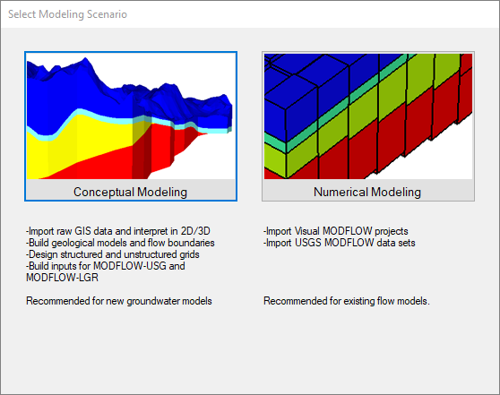
•Select [Numerical Modeling] and the Numerical Modeling workflow will load.
•The first step is to Define Modeling Objectives.
Define Modeling Objectives
•In this step, you define the objectives of your model and the default parameters.
•The Start Date of the model corresponds to the beginning of the simulation time period.
•Select 1/1/2000 for the Start Date
•For this scenario, we will include contaminant transport in the model run. Click the check box beside 'Transport Active' (in the right hand side of the window, under Define Modeling Objectives.
•For 'Retardation Model' select 'Linear isotherm (equilibrium-controlled)'. For this tutorial you will not be simulating any decay or degradation of the contaminant, so the default 'Reaction' setting of 'No kinetic reactions' will be fine.
•Below the 'Retardation Model' and 'Reaction' settings are two tabs: 'Species Parameters' and 'Model Parameters'. By default, one species (chemical component) is defined for the transport run. For this example, we will leave the initial concentration ('InitialConcentration (mg/L)') as zero, but adjust Kd (the distribution coefficient)
•Type 1E-7 in [Kd 1/(mg/L)] column
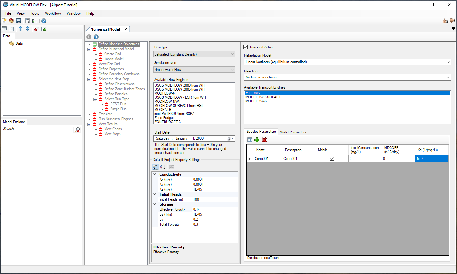
•You are now finished setting up the flow and transport objectives. Click [![]() ] (Next Step) to proceed.
] (Next Step) to proceed.
•The following 'Define Numerical Model' step will appear; at this step, you can import Visual MODFLOW Classic or MODFLOW data sets, or define a new empty grid. For this tutorial we will create a new grid.
•Click on [Create Grid] to proceed

Create Grid
•At this step, you can specify the dimensions of the Model Domain, and define the number of rows, columns, and layers for the finite difference grid. Type the following into the Grid Size section,
•Columns: 40
•Rows: 40
•For Grid Extents, enter 2000 for Xmax and 2000 for Ymax
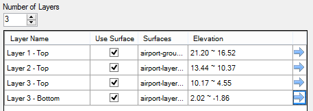
•Under Define Vertical Grid, Type 3 for Number of Layers
Define Layer Elevations
•In Visual MODFLOW Flex, you can define the elevations of the tops and bottom of the model layers. Or you can have varying layer elevations defined from Surface data objects. Surfaces could be from data objects you imported from Surfer (.GRD, ESRI .ASI, .DEM), or from Surfaces you have created through interpolating XYZ points. In this exercise, you will import 4 surfaces (from Surfer .GRD files), then use these to define the layer elevations.
•Click [File] then [Import Data...] from the main menu. The following window will appear:

•For the Data Type, select 'Surface' from the drop-down list.
•In the Source File field click the […] button and navigate to C:\Users\Public\Documents\Visual MODFLOW Flex\Tutorials\Airport\suppfiles\Surfer\airport-ground-surface.grd and select [Open]
•Click [Next>>]
•Click [Next>>] (accept the defaults)
•Click [Next>>] (accept the defaults)
•Click [Finish]. You should now see a new "airport-ground-surface" data object appear in the data tree, in the top left corner of the window.
•Now, repeat the above steps to import the other Surfer .GRD files into the project:
oairport-layer2-top.grd
oairport-layer3-top.grd
oairport-layer3-bottom.grd
•When you are finished, you should see 4 Surface data objects in the data tree in the top left corner.

•Now you are ready to define the grid layers using these surfaces. Under Number of Layers, select 'Use Surface' check box for each grid layer. This is shown below

•Next you will provide a surface for each layer;
•Click on airport-ground-surface from the data object tree (it should become selected), then click on the topmost blue arrow [![]() ] beside 'Use Surface' in the Number of Layers table (in the row that starts "Layer 1 - Top". If you have done this correctly, the table should appear as shown below.
] beside 'Use Surface' in the Number of Layers table (in the row that starts "Layer 1 - Top". If you have done this correctly, the table should appear as shown below.

•Now repeat these steps for the remaining layers:
•Select airport-layer2-top Surface data object to the tree, and insert this (using the [
![]()
]) as the Surface for Layer 2 - Top
•Select airport-layer3-top Surface data object to the tree, and insert this (using the [
![]()
]) as the Surface for Layer 3 - Top
•Select airport-layer3-bottom Surface data object to the tree, and insert this (using the [
![]()
]) as the Surface for Layer 3 - Bottom
•When you are finished, the table should appear as shown below.
•You are finished defining the layer elevations.
•Click on the [Create Grid] button (near the top right of the window) to create the grid. You will see the model tree will be generated on the left side of the window in the Model Explorer, and 'NumericGrid1' should appear as the last item.
•Click on the next button [
![]()
] to proceed to View/Edit Grid step.
Refine the Grid
This section describes the steps necessary to refine the model grid in areas of interest, such as around the water supply wells, refueling area, and area of discontinuous aquitard. The reason for refining the grid is to get more detailed simulation results in areas of interest, or in zones where you anticipate steep hydraulic gradients. For example, if drawdown is occurring around the well, the water table will have a smoother surface if you use a finer grid spacing. Also, layer properties can be assigned more correctly on a finer grid.
•Right click on the 'NumericalGrid1' from the tree, and select [Edit Numerical Grid...] (Alternatively, select Edit grid... in the View/Edit Grid step).
•The following window will appear:

The grid refinement works by defining a starting row number, and ending row number, then a 'Refine by' factor; to help you define the limits of where the refinement should be applied, you can add data objects to this display, such as well locations, arial maps, shapefiles, etc. When you are using this feature with your own models, you will need to import these data object files before starting the 'Grid Refinement' step.
•You will first start by refining the rows.
•Enter '5' in the 'From' field, and enter '35' in the 'To' field.
•Enter 'Replace Every [1] row(s) with [2]'. Your screen should appear as follows:
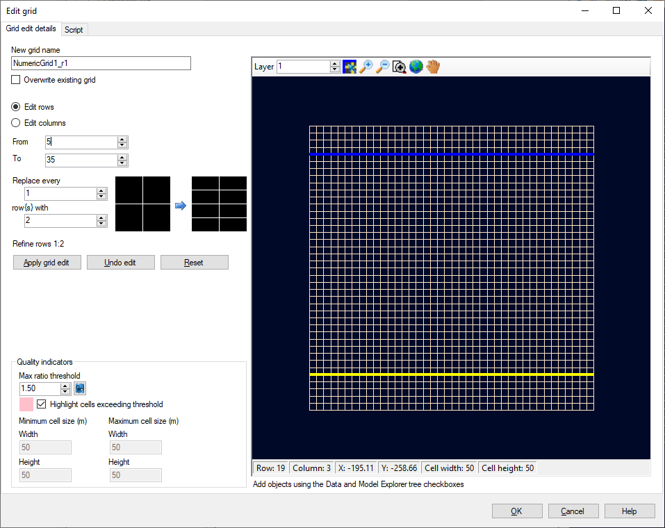
•Click on the [Apply grid edit] button.
•Next, you will refine the columns.
•At the top left of the window, select the [Edit Columns] radio button.
•As before, Enter '5' in the 'From' field, and enter '35' in the 'To' field.
•Enter Replace every [1] column(s) with [2]
•Click on the [Apply grid edit] button.
You should now see coarse grid sizes around the edge of the model domain, and a more finer sized grid spacing in the middle of model (around the areas interest). This is shown below. The band of pink cells around the edges of the refinement indicate cells where the Max ratio threshold quality indicator (which is set by default to a cell step size of 1.50) has been exceeded. Large aspect ratios between cells can sometimes result in longer computation times, decreased stability, and increased numerical error. These areas can be further fractionally refined to improve the grid quality; in this exercise, we will leave the grid as-is and proceed to the next step.

•Click on the [OK] button.
In the Model Explorer tree, a new grid and numeric workflow (i.e. 'NumericGrid1_r1') is created, and a new workflow window/tab (i.e. 'NumericGrid1_r1-Run1') opens. At this stage we will continue working with the refined grid, and we can ignore the initial coarse grid.
•In the next section, you will view the numerical grid that you just created.
•Click on the Define Properties step or click the next button [
![]()
] to proceed.
Define Flow Properties
This section will guide you through the steps necessary to design a model with layers of highly contrasting hydraulic conductivities.
•First, ensure that 'Conductivity' is selected in the first dropdown menu under the 'Toolbox'
•Click on the [Edit...] button and Type the following values in the top row of the window:
oKx (m/s): 2E-4, then use [F2] to propagate through all cells
oKy (m/s): 2E-4, then use [F2] to propagate through all cells
oKz (m/s): 2E-4, then use [F2] to propagate through all cells
•Click [OK] to accept these values.
In this case the Kx, Ky, and Kz values are the same, indicating the assigned property values are assumed horizontally and vertically isotropic. However, anisotropic property values can be assigned to a model by modifying the Conductivity Database.
In this three layer model:
•Layer 1 represents the upper aquifer
•Layer 2 represents the aquitard separating the upper and lower aquifers, and
•Layer 3 represents the lower aquifer.
For this example, we will use the previously assigned hydraulic conductivity values (Zone# 1) for model layers 1 and 3 (representing the aquifers) and assign different Conductivity values (i.e. a new Zone) for model layer 2 (representing the aquitard). Note that layer 1 is the top model layer.
•Next you need to change to Layer 2. (using the up arrow under the Layer text box shown below)

You are now viewing the second model layer, representing the aquitard. The next step in this tutorial is to assign a lower hydraulic conductivity value to the aquitard (layer 2). We can graphically assign the property values to the model grid cells.
•Click [Assign] then [Entire Layer/Row/Column] from the toolbox.
The following dialog will appear:

•Click on the [New] button at the top; this will create a new zone.
•Enter the following values:
oKx (m/s): 1E-10
oKy (m/s): 1E-10
oKz (m/s): 1E-11
The dialog should appear as shown below:

• Click [OK] to accept these values.
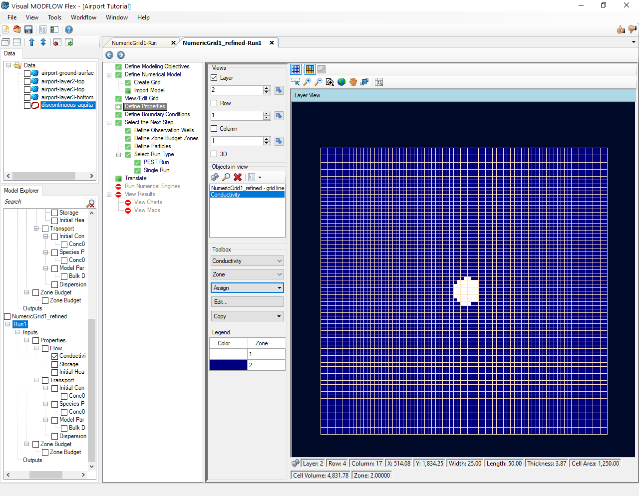
Once finished, the cells for Layer2 should change blue, which indicates these cells belong to Zone2; you can use the Legend under the toolbox as a guide, and also mouse over cells in the grid view, and note the values in the status bar.

Next you must assign the appropriate conductivity values to the discontinuous region. Although the region where the aquitard pinches out is very thin, the conductivity values of these grid cells should be set equal to the Conductivity values of either the upper or lower aquifers.In this particular example, the zone of discontinuous aquitard is indicated on a shapefile. We will import this shapefile into the project:
•Click [File] then [Import data...]
•For the Data Type, select Polygon from the drop-down list.
•In the Source File field click the […] button and navigate to your Public "My Documents" folder, then 'VMODFlex\Tutorials\Airport\suppfiles\discontinuous-aquitard.shp', and click [Open]
•Click [Next>>]
•Click [Next>>] (accept the defaults)
•Click [Next>>] (accept the defaults)
•Click [Finish].
•You should now see a new data object, 'discontinuous-aquitard' appear in the data tree, in the top left corner of the window.
•Click on the box beside this data object in the tree
![]()
.
•The data object should now appear in the Layer View of the grid.
•Zoom into this area (using the mouse wheel, or the Zoom in button on the toolbar).
•Click [Assign] then [Using Data Object] from the toolbox.
•Use the [
![]()
] button to pull in the discontinuous-aquitard shape file in the new property zone window (you can also drag/drop a data file into this field)
•We want to assign these cells to an existing Zone: Zone1 that represents the aquifer above. So in this case, it is not necessary to create a new parameter zone. Use the zone arrows to select Zone 1 and verify that the K-values are all 0.0002 and that Layer 2 is selected (i.e. the checkbox for layer 2 is checked in the 'Assign to Layers' section). Your screen should look like the following:

•Click [OK] to assign this group of cells to Zone1. This display should appear as shown below.
•Now view the model in cross-section to see the three hydrogeological units. First, zoom out to the fill extent using one of the following options:
| •
Zoom out button from the toolbar |
| •
Zoom full extents button from the toolbar •Scroll wheel on the mouse (scroll forwards) |
•Click the [Column] check box in the 'Views' section. You will see another view appear beside the layer view, showing a cross-section through the model domain (by default, through Column1). To improve this view, you should change the Exaggeration
•Enter 40 in the Exaggeration field, which is located in the toolbar directly above the Column view window.
•Enter 37 for the Column number, as this will provide a cross-section through the region with the discontinuous aquitard. Take a moment to view the cross-section of the properties. You can also change the cross-section view (change the Column number up, down, or enter a new value), and use the zoom and pan tools on the Column view to improve the display. Note that you can repeat the same steps above for Rows, instead of Columns, in order to see cross-sections along the X-axis.
•The display should look similar to the image below:

•When you are finished, turn the Column View off, by removing the check-box beside [Column] under 'Views'.
•Now is a good time to save the project. Click [File] then [Save Project] from the main menu.
•Click [
![]()
] (Next Step) to proceed.
Define Boundary Conditions
The next step is to define the flow boundaries for the model. In this example, you will define:
•constant heads along the north edge of the model domain in layers 1 and 3,
•the Waterloo River along the southern portion of the model in layer 1,
•a constant head along the southern edge of the model in layer 3, and
•two recharge zones with differing rates applied at the top of the model (ground surface)
You will also import and define pumping wells in the next section of this tutorial.
Constant Heads
The first Constant Head boundary condition will be for the upper unconfined aquifer along the northern boundary of the model domain. To do this you will use the [Assign]>[Polyline] tool.
•First, you need to go back to Layer 1. Type '1' into the [Layer] field under 'Views' (or use the arrow buttons).
•Next, ensure that 'Constant Head' is selected from the first dropdown menu under the 'Toolbox' section.
•Under the 'Toolbox' section, click [Assign]>[Polyline]. Move the mouse pointer to the north-west corner of the grid (top-left grid cell) and left-click on this location to anchor the starting point of the line. Now move the mouse pointer to the north-east corner of the grid (top-right grid cell) and Right-Click on this location to indicate the end point of the line. Click 'Finish', then you should then see a small menu appear to 'Define Boundary Condition'.
•Click [Next >>] to accept the default name.
•Enter Starting Head (m) of 19 in the top row and hit F2 to propagate this value.
•Enter Ending Head (m) of 19 in the top row and hit F2 to propagate this value.
•Leave the default value of -1 for Conc001; this indicates that no contaminant mass will be assigned to these cells.

•Click [Finish] to complete the boundary condition. The hand-drawn polyline will now turn to a set of red points, indicating that a Constant Head boundary condition has been assigned to these cells. The display should look like the image below:

Next you will assign a Constant Head boundary condition along the northern boundary for the lower confined aquifer.
•Locate the [Layer] selection in the 'Views' section, and change this to '3'.

•Ensure that 'Constant Head' is still selected from the first menu under the 'Toolbox' section.
•Click [Assign]>[Polyline] from the toolbox. Move the mouse pointer to the north-west corner of the grid (top-left grid cell) and left-click on this location to anchor the starting point of the line. Now move the mouse pointer to the north-east corner of the grid (top-right grid cell) and right-click on this location to indicate the end point of the line. Click 'Finish' then you should then see a small menu appear 'Define Boundary Condition'.
•Click [Next >>] to accept the default name.
•In the Define Boundary Condition dialog, enter the following values:
•Enter Starting Head (m) of '18' in the top row and hit F2 to propagate this value.
•Enter Ending Head (m) of '18' in the top row and hit F2 to propagate this value.
•Click [Finish] to complete the boundary condition. The hand-drawn polyline will now turn to a set of red points, indicating that a Constant Head boundary condition has been assigned to these cells
Next, assign the Constant Head boundary condition to the lower confined aquifer along the southern boundary of the model domain.
•Click [Assign]>[Polyline] from the toolbox. Move the mouse pointer to the south-west corner of the grid (bottom-left grid cell) and click on this location to anchor the starting point of the line. Now move the mouse pointer to the south-east corner of the grid (bottom-right grid cell) and right-click on this location to indicate the end point of the line. Click 'Finish' then you should then see a small menu appear 'Define Boundary Condition'.
•Click [Next >>] to accept the default name.
•In the Define Boundary Condition dialog, enter the following values:
•Enter Starting Head (m) of '16.5' in the top row and hit F2 to propagate this value
•Enter Ending Head (m) of '16.5' in the top row and hit F2 to propagate this value.
•Click [Finish] to complete the boundary condition. The hand-drawn polyline will now turn to a set of red points, indicating that a Constant Head boundary condition has been assigned to these cells
River
The following instructions describe how to assign a River boundary condition in the top layer of the model, along the southern edge of the model.
•First, you need to go back to Layer 1. Type '1' into the [Layer] field under 'Views' (or use the arrow buttons).
•Now we need to import our river data object (using the steps explained previously; [File]>[Import Data]>'Polyline'>'river.shp')
•Select 'River' from the first dropdown menu in the 'Toolbox' section.
•Click [Assign]>[Using Data Object] from the toolbox. Use the [
![]()
] button to add the river data object to the geometry section of the 'Define Boundary Condition' dialog. Hit [OK] to the message that the extents will be clipped to the model domain.
•Click [Next>>] to accept the default name.
•The 'Define Boundary Condition' window will appear as shown below.
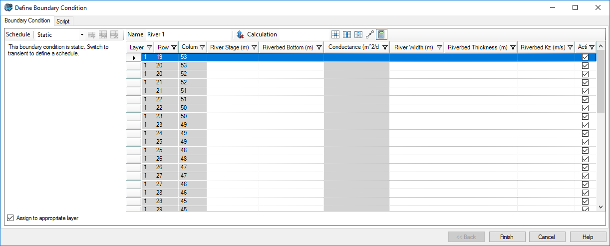
Traditionally, the River boundary condition has required a value for the conductance of the riverbed. However, the conductance value for each grid cell depends on the length and width of the river as it passes through each grid cell. Therefore, in a model such as this, with different sizes of grid cells, the conductance value will change depending on the size of the grid cell. In order to accommodate this type of scenario, Visual MODFLOW Flex allows you to enter the actual physical dimensions of the river at the Start point and End point of the line, and then calculates the appropriate conductance value for each grid cell according to the standard formula.
Select the first row in the define Boundary Condition dialog and notice Flex has highlighted in yellow the corresponding river cell (lower left corner of the river). This dialog is interactive; you can select cells in the dialog or viewer/grid window to see how boundary values are currently assigned.
•In the top row of the boundary assignment dialog enter the following values for the start point.
| River Stage (m) | 16.0 |
| Riverbed Bottom (m) | 15.5 |
| Conductance (m^2/day) | (automatically calculated based on width, thickness and Kz) |
| River Width (m) | 25 |
| Riverbed Thickness (m) | 0.1 |
| Riverbed Kz (m/s) | 1E-4 |
|
| Leakance from the river will be calculated based on the parameters you define. For more details on the calculation, refer to Boundary Conditions Theory |
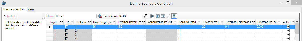
•Now you will define the values for the End Point of the river.
•Scroll to the bottom row in the Define Boundary Condition dialog and click in it. Notice the river end cell is now highlighted yellow in the grid view.
•Now define the values at this end point, in the parameters grid, based on the values below:
| River Stage (m) | 15.5 |
| Riverbed Bottom (m) | 15.0 |
| Conductance (m2/d) | (do not enter any values) |
| River Width (m) | 25 |
| Riverbed Thickness (m) | 0.1 |
| Riverbed Conductivity (m/s) | 1E-4 |
•We will now linearly interpolate the intermediate values. To do this:
•Click the grey box next to the top (start) row to highlight the whole row blue as shown below:
•Holding the CTRL key on your keyboard, click to also highlight the last (end) row.
•Now click the interpolate button [
![]()
]. The intermediate rows should now populate with interpolated values.
•Click [Finish] to complete the boundary condition. The polyline will now turn to a set of blue points, indicating that a River boundary condition has been assigned to these cells. The interface should now look like the image below:

Recharge
In many hydrogeologic settings, aquifers are recharged by water infiltrating from the land surface. In order to assign recharge in Visual MODFLOW Flex, you must be viewing the top layer of the model. Check the 'Views' frame in the upper left-hand side of the main workflow window to see which layer you are currently in. The first boundary condition to assign is the recharge flux to the aquifer:
•First, you need ensure you are viewing Layer 1. Type '1' into the [Layer] field under 'Views' (or use the arrow buttons).
•Select 'Recharge' from the list of boundary conditions in the toolbox.
•Click [Assign]>[Entire Layer] from the toolbox. The 'Define Boundary Condition' dialog will appear.
•Click [Next >>] to accept the default name.
•Enter 100 in the 'Recharge (mm/yr)' column and hit F2 to propagate this value to all rows.
•Leave the default value of -1 for Conc001; this indicates that no contaminant mass will be assigned to the recharge flux.
•Enter 0 in the 'Ponding (m)' column and hit F2 to propagate this value to all rows, as shown below. The Ponding parameter is not used by any engine except MODFLOW-SURFACT, so for models not using this engine this parameter has no effect.
•Finally, change the Schedule from 'Transient' to 'Static'
•The Define Boundary Condition window should now look like the image below:

•Click [Finish]. All cells in the top layer will be assigned a recharge rate of 100 (mm/yr). The recharge boundary will be displayed as white dots.
Now you will assign a higher recharge value at the Refueling Area where jet fuel has been spilled on a daily basis. First you need to import a polygon shapefile that delineates this area.
•Click [File]>[Import data...]
•For the Data Type, select 'Polygon' from the drop-down list.
•In the Source File field click the […] button and navigate to your Public "My Documents" folder, then 'VMODFlex\Tutorials\Airport\suppfiles\refuelling-area.shp', and click [Open]
•Click [Next>>]
•Click [Next>>] (accept the defaults)
•Click [Next>>] (accept the defaults)
•Click [Finish]. You should now see a new data object, 'refuelling-area' appear in the data tree, in the top left corner of the window.
•Click on the box beside this data object in the tree
![]()
. The data object should now appear in the Layer View of the grid (it is located in the top middle of the site).
![]() Please Note: you may need to uncheck 'Recharge' from the Model Explorer tree to make the view less cluttered.
Please Note: you may need to uncheck 'Recharge' from the Model Explorer tree to make the view less cluttered.
•Zoom into this area (using the mouse wheel, or the Zoom in button on the toolbar).
•Click [Assign]>[Using Data Object...] from the toolbox. A 'Define Boundary Condition' window will appear. Use the [![]() ] button to add the 'refuelling-area' object to the geometry section of the dialog.
] button to add the 'refuelling-area' object to the geometry section of the dialog.
•Click [Next >>] to accept the default name.
•Enter 250 in the 'Recharge (mm/yr)' column and hit F2 to propagate this value to all rows.
•Enter 0 in the 'Ponding (m)' column and hit F2 to propagate this value to all rows.
•Finally, change the Schedule from 'Transient' to 'Static'
•Notice that Conc001 has a default of -1 indicating that there is no defined mass flux assigned to this boundary condition. You will modify this later on in the Transport section of the tutorial.

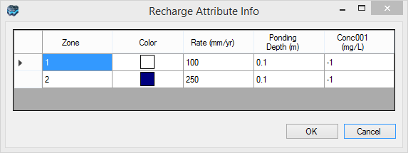
•Click [Finish]. You should now see a new zone of cells colored blue, indicating the new RechargeZone2, with this new value
•Click [Database] to see the recharge zones you created, and their corresponding values.
•Click [OK] to close the window
•Now is a good time to save the project. Click [File]>[Save Project] from the main menu.
Define Pumping Wells
To generate a pumping well boundary condition, you can either add them one at a time through the user interface, or use a wells data object for this model, you will begin by importing a wells data object.
•Click [File]>[Import Data...] from the main menu.
•Select 'Well' as the data type.
•[…] to choose the source file
•Browse to your Public "My Documents" folder, then 'Visual MODFLOW Flex\Tutorials\Airport\suppfiles\Pumping_Wells.xlsx' file.
•[Open]
•[Next>>]. The next window will show a preview of the data to be imported.
•[Next>>].
•VMOD Flex provides you with various options to import well data. In this window, you must select to import the well heads, screens, and pumping schedules.
•Select the Well heads with the following data option button.
•Select the Pumping schedule checkbox.

•[Next>>]
•[Next>>] to accept the default Coordinate System.
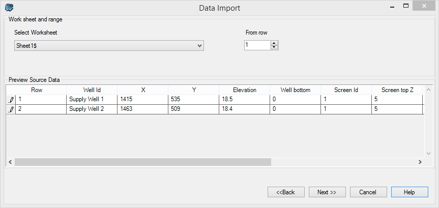
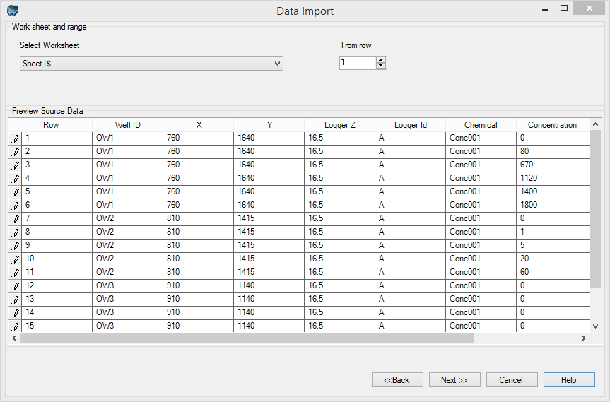
The following 'Data Import' window will then appear:

In this screen, you need to map the fields from the spreadsheet to required fields in the data import utility. If you prepare your Excel file with the exact column names that are expected by Visual MODFLOW Flex, then no mapping is required and this can save you time. For this exercise, the source Excel file has the map names pre-defined. Take a moment to review the required fields for the Wells import:
•Well heads: Well ID, XY Coordinates, Elevation, and Bottom
•Screens: Screen Id, Screen top Z, Screen bottom Z
•Pump Schedule: Pumping start date, Pumping end date, Pumping rate
|
| When working with your own pumping well data for your models, you can use this Excel file as a template – having all the fields automatically mapped for you reduces the effort required during the import process, and minimizes sources of error. |
Switch to the Screens Tab to see the mapped fields:

•Click [Next>>].
The Data Import preview will appear:

•You should see a series of green check marks next to the 'Heads', 'Screens' and 'Pump Schedule' tabs indicating that there were no import errors.
•Click [Finish].
The 'Pumping_Wells' will now appear as a new data object in the Data tree.
Next, you need to add the imported wells to the Numerical Model
•At the Define Boundary Conditions step in the workflow, under Toolbox, choose 'Wells' from the first dropdown menu listing available boundary condition types.
•Click the [Assign]>[Using Data Object] button. An 'Add Wells' window will appear.
•Select (highlight) the 'Pumping_Wells' data object from the Data Tree (you may need to move the Pumping Wells Boundary Condition dialog to the right in order to see this).
•Click [
![]()
] button located in the middle of the 'Create Well Boundary Condition' window, under 'Select Raw Wells Data Object or Drag & Drop'. Once completed, your display should appear as shown below.

•Click [OK]. The pumping wells have now be added to the numerical model.
You should see a new node appear on the Model Explorer, under 'NumericGrid1_r1/Run/Inputs/Boundary Conditions/Wells'. In order to see these wells, you need to turn off the Recharge coverage and change to Layer 3.
•Click on the box beside 'Recharge' in the Model Explorer, to remove the check box
•Change to Layer 3 (as explained earlier).
•Also, you may need to zoom out to the full grid extents, by selecting the [
![]()
] (Zoom to Full Extents) button on the toolbar above the grid.
•You should see the two points representing the wells, located in the lower right corner of the model domain, as shown in the following figure.

•Now is a good time to save the project. Click [File]>[Save Project] from the main menu.
Define Head Observations
Field observations of groundwater heads and fluxes are essential in order to calibrate the results obtained by MODFLOW. In this exercise, you will add several head observations wells, and analyze these against the corresponding calculated values after the model run is complete. The head observations are grouped into two files, one for layer 1 (observation wells 1-5) and another for layer 3 (observation wells 6-10). First we need to import the observation wells:
•Click [File]>[Import Data] from the main menu bar
•Ensure 'Well' is selected as the Data Type
•[…] to choose the source file.
•Browse to your Public 'My Documents' folder, then 'Visual MODFLOW Flex\Tutorials\Airport\suppfiles\Head_Observations_Layer1.xlsx' file.
•[Open]
•[Next>>]
A preview window will appear displaying the source data.

•[Next>>]. VMOD Flex provides you with various options to import well data.
•Choose the radio button [Well heads with the following data]
•Then select [Observations points]
•Then select [Observed heads]
•Ensure you have the options selected as shown below.

•[Next>>]
•[Next>>] to accept the default Coordinate System
In this screen, you need to map the fields from the spreadsheet to required fields in the Wells Import utility.
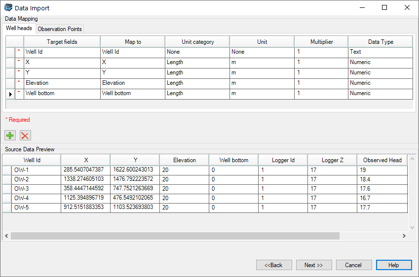
To save time, you can prepare your Excel file with the exact field names that are required by Visual MODFLOW Flex, and then no mapping is required. For this exercise, the source Excel file has the field names pre-defined for automatic mapping and can be used as a template/guide for your other projects. Take a moment to review the required fields for the Wells import:
•Well heads: Well ID, XY Coordinates, Elevation, and Bottom
•Observation points: Logger Id, Logger Z, Head observation date, Observed head
•[Next>>]
The Data Import preview will appear, indicating if there were any errors with the file import. This file should import with no errors.
•[Finish]
The 'Heads_Observations_Layer1' will now appear as a new data object in the Data Tree. Take a moment and visualize this in the 3D Viewer.
Next you need to add these raw observation wells as observation points for the numerical model.
•Click [
![]()
] (Next Step) to proceed.
•Select Define Observations
•Next, ensure that 'Well Observation' is selected from the first dropdown menu under the 'Toolbox' section.
•Be sure that the 'Head_Observations_Layer1' data object is selected in the Data Tree.
•Click [Assign]>[Using Data Object] from the toolbox. Click on the [
![]()
] button to add the Well Observation object.
•Ensure you have the options selected as shown below.
•Click [OK]. The observation wells will be added to the display and the numerical model tree.
You should see several green points in the model domain that represent the locations where head measurements were taken. Note that all of the head observations added so far are in layer 1.

Now you will repeat these steps to import the observation wells for layer 3 of the model. Follow the same steps above, but this time import the 'Head_Observations_Layer3.xlsx' file. When you import a second observation group, you will be prompted to assign the observations "...to an existing well group", or to "... a new well group', as indicated in the image below:

•Click 'Assign observations to a new well group'
•OK
Once the observations for layer 3 have been imported you can view them in layer 3, as shown below:

•Now is a good time to save the project. Click [File]>[Save Project] from the main menu.
•Click [
![]()
] (Next Step) to proceed.
Select Run Type and Engines
At this step in the tutorial, you select which engine(s) to run in the simulations:
•In the 'Select Run Type' step, select [Single Run]
•From the 'Single Run' step in the workflow, you will see 'USGS MODFLOW 2005 from WH' is selected along with 'MT3DMS' as the transport engine.
•For the first run, we will run the flow solution only, without transport.
•Deselect the checkbox for 'Run Transport Engine'
•Click [
![]()
] (Next Step) to proceed.
MODFLOW-2005 Translation Settings
At the Translate step you have the option to adjust the various parameters and flags for the MODFLOW packages and run time settings. Available options include: 'Settings' (General), 'Settings' (MODFLOW-2005), 'Solvers', 'Recharge and Evapotranspiration', 'Lake', 'Layers', 'Rewetting', 'Initial Heads', 'Anisotropy', 'Output Control' and 'Advanced Settings'.
•Select [MODFLOW-2005]>[Settings]
•Enter 7300 for 'Steady-State Simulation Time' (in the grid in the main window). Note that this value does not affect the simulation results, as steady-state models are always run to equilibrium. The Steady-State Simulation Time is simply a multiple on the reported mass balance values; here we are specifying that we want 7300 day (~20 year) water budgets.

•Click [
![]()
] to create the MODFLOW-2005 packages. Check the log to confirm the translation has finished.

•Click [
![]()
] (Next Step) to proceed.
Run MODFLOW-2005
At this step in the tutorial, you will run the model:
•Click the [
![]()
] button to run MODFLOW-2005.
The model run should complete in a few seconds. Once finished, you should see the message: "The run was successful" in the engine progress window. In addition, you will see several items will be added to the model tree under 'Output', as shown below:
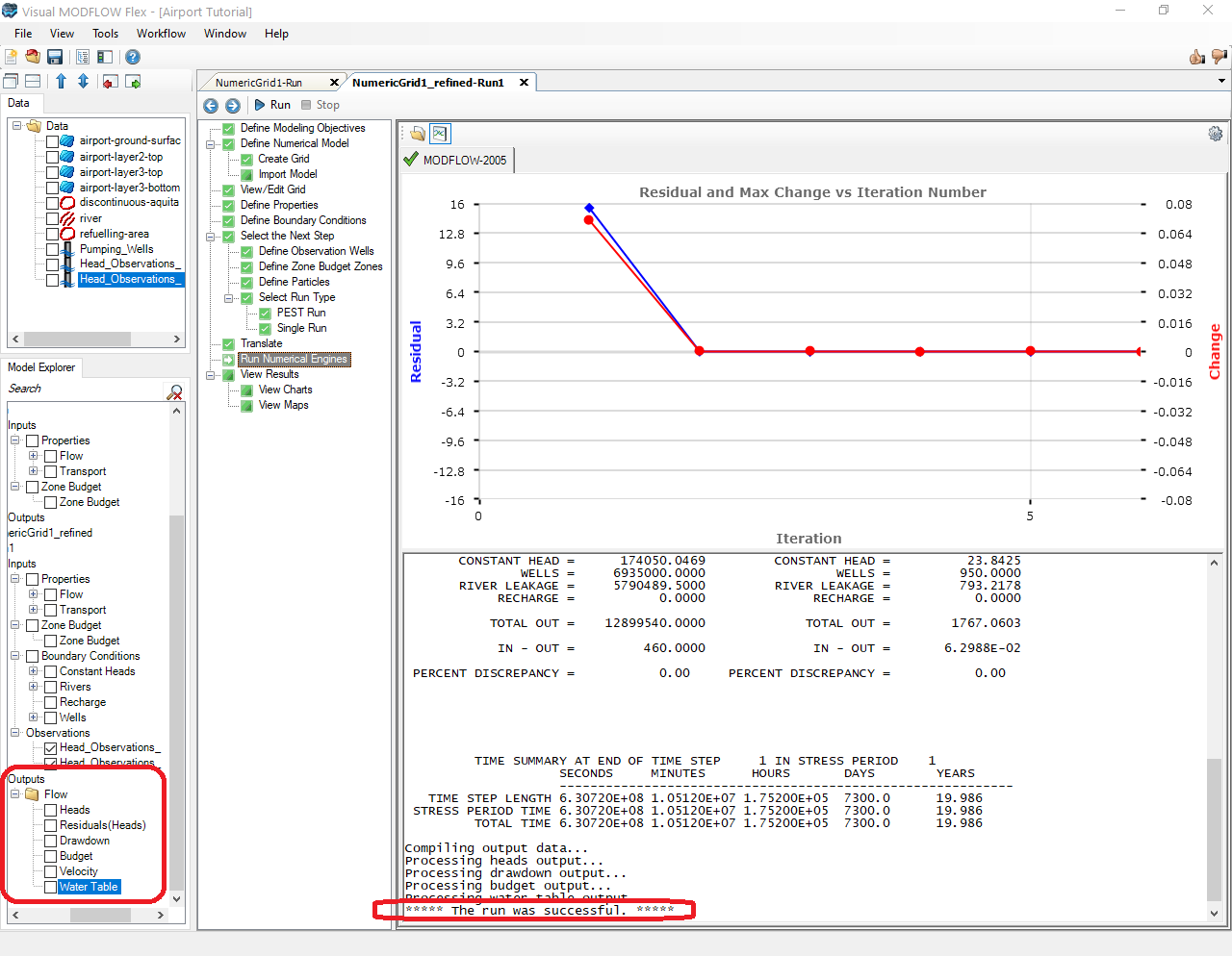
•Now is a good time to save the project. Click [File]>[Save Project] from the main menu.
•Click [
![]()
] (Next Step) to proceed.
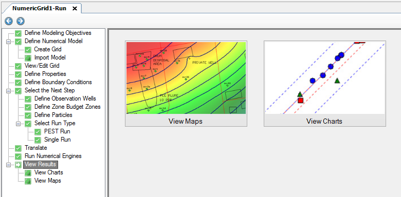
View Maps (Heads, Velocities and Calibration Residuals)
The following 'View Results' window will then appear; you have the option to View Maps or View Charts. We will start by viewing maps of heads.
Heads
The standard display at the View Maps step includes a visualization of the output simulated head distribution. To display the simulated heads do the following:
•Click [View Maps] button to proceed. You will then see color shading of the calculated heads, in layer view. You can press F4 to hide the workflow, and bring it back again at any time by pressing F4 again.

•If you do not like the default contour interval or line color, you can customize the contour map settings.
•To access the contouring options for Heads, right-click on 'Heads' from the model tree, and select [Settings...]. The following dialog will appear

•From the Settings tree on the left, select 'Style' followed by 'Contour Lines'. This will expand the settings window and give you access to the Contour Line settings.
•Under 'Automatic contour', enter 0.2 for the contour interval, and start/finish the contour at 12/20. This is shown below:
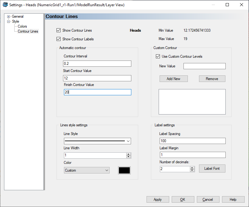
•When you are finished, click [OK].
•This will apply the changes to the head contours in your current view.
|
Preview Display Settings before Committing |
| All of the Settings windows have an [Apply] button in the lower right corner. This means you can apply the adjusted changes and see the impact in the current 2D or 3D view before you close the window. This makes it easier to obtain the desired display without having to open and close this window numerous times. |
•You can also display heads along a row, along a column, or in 3D using the same tools that you used earlier.
•In the 'Views' section activate the 3D view and deactivate the layer view. Apply an exaggeration of 40 and reorient your view so that you can see head values along a layer, column and row. You should see something similar to the image below:
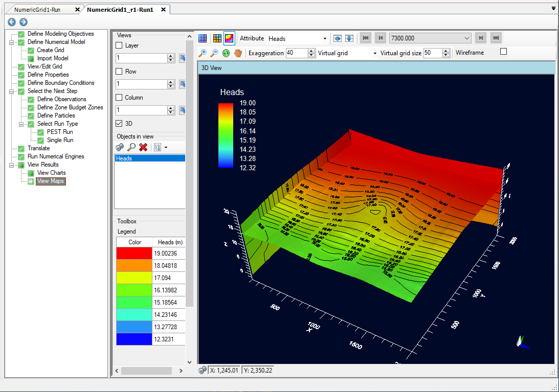
•Take a moment to view the heads in other layers/rows/columns.
Velocity Vectors
It is also possible to visualize the results of your flow model as a distribution of velocity vectors, which allows you to easily display and interpret flow fields. To display a velocity map do the following:
•First, ensure you are viewing 'Layer 3'. This layer contains the pumping well, and should contain a significant flow field in that region.
•Turn off the check box beside 'Heads' in the Model Explorer
•Turn on the 'Velocity' output option, in the Model Explorer under 'Outputs' > 'Flow'
•Access the Velocity display settings by right-clicking and selecting 'Settings'
•In the Settings window, access the 'Style' > 'VelocityMap' settings
The VelocityMap settings window should appear as below:

Velocity vectors may be displayed using average linear or Darcy velocities. In-plane velocity vectors can be displayed using the full magnitude of the vector (i.e. the out-of-plane velocity component will be included), as a projection (i.e. only the in-plane velocity component is displayed), or simply a directional indicator (i.e. the size of the arrow is not dependent on the actual velocity). By default, the velocity vectors will initially be displayed as a projection with average linear velocity values, on a linear scale.
A normal velocity color map function is also supported, which allows you to interpret flows perpendicular to the selected layer/row/column (i.e. out-of-plane flow). By default the normal velocity color map will be displayed with a red/blue color scheme, with red areas indicating flow inward (i.e. corresponding to the positive X, Y or Z direction), and blue areas indicating flow outward (i.e. corresponding to the negative X, Y or Z direction). Areas with velocities below the specified in-plane range threshold will be displayed using the specified In-plane color (which is grey by default). You can find more information about the velocity map display settings in the 3D Gridded Data section of this manual.
Update the velocity map settings as follows:
•In the 'Color' frame, select the 'Custom' option, and select 'Orange' as the display color
•In the 'Velocity type' frame, select the 'Average Linear' option
•In the 'Scale factor' frame, type a scale factor of 3.0
•Deselect the 'Show legend' option, so that the legend will be hidden
•Once these settings have been applied, the Layer view should look like the image below (Layer 3)

You should be able to see larger velocity vectors in the bottom-right corner of the model, in the vicinity of the pumping wells. These indicate that groundwater flows are significantly faster in this area relative to the rest of the model domain. You may also notice a 'ring' approximately in the middle of the model. This indicates that there is significant flow perpendicular to layer 3 in this zone. Since the ring is blue, that would indicate flow in the negative Z direction, or downwards from layer 2 and into layer 3.
Calibration Residuals
It is also possible to visualize the results of your flow model as a distribution of residuals, provided you have associated observations. This allows you to easily display and interpret the spatial distribution of the differences between observed and simulated heads. To display a residuals map, do the following:
•First, off the 'Velocity' output option, in the Model Explorer under 'Outputs' > 'Flow'
•Next, turn on the 'Heads' and 'Residuals(Heads) output options, in the Model Explorer under 'Outputs' > 'Flow'
The residuals are shown in the map as a series of error bars. The target residual interval (default = 1 unit of length measurement, typically feet or meters) is shown as a set of three parallel black bars. The residual value is shown as a filled column colored and color coded by whether the residual exceeds the target interval above (blue) or below (red) the observed value or lies within one target interval (green). By default, only the residuals in the current slice (layer/row/column) will be shown. You can experiment with showing residuals differently by changing the ResidualsMap style settings, which can be accessed by right-clicking on the Residuals in the Model Explorer tree.
The Residuals Map settings window should appear as below:

View Charts (Heads)
It's very easy to review calibration charts in Visual MODFLOW Flex whenever observation data has been applied to your model. Since we have applied observed head values in a previous step, we can now proceed to the 'View Charts' workflow step to view the automatically generated calibration charts.
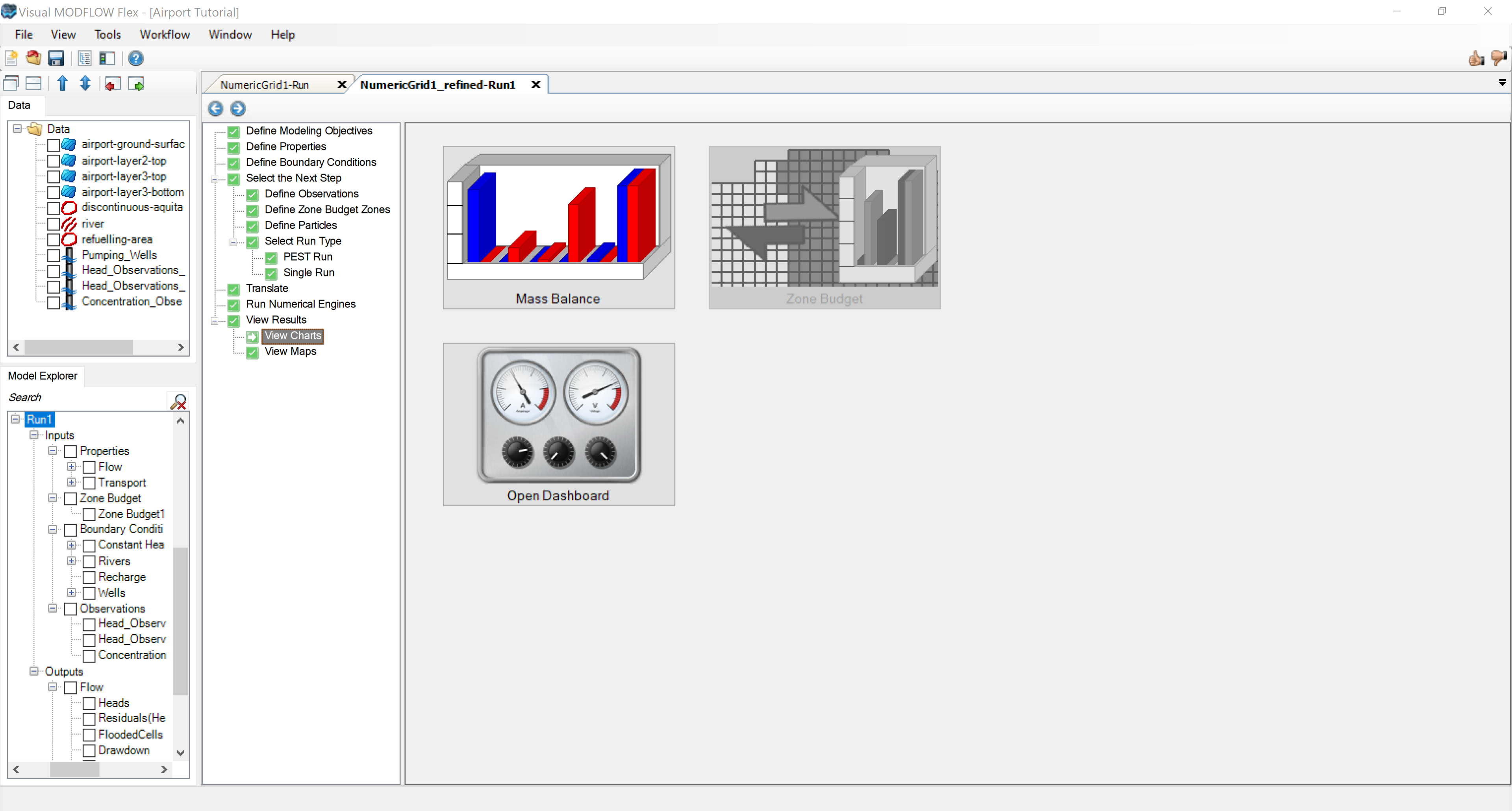
•Click 'View Charts' from the workflow tree. You can open the Mass Balance, Zone Budget, or Open Dashboard at this step. For this tutorial, we will click on Open Dashboard.
•Click [Open Dashboard] to proceed.
As you can see from the image below, Visual MODFLOW Flex supports a number of methods for selecting different wells and provides flexible settings to show/hide wells using filters in the observation data table (show in red below), such as: model layer, observation groups, conductivity zone. Data on the dashboard chart(s) are automatically updated and displayed based on the applied filters.

Next, apply a filter to the model layers so that only observations in Layer 1 are shown:
•Select the dropdown button in the first row of the table for the Layer field and click [
![]()
] to select a filter from the Attribute Table. Note, you may wish to expand the table by clicking and dragging the separation line between the table and the chart to the right.
•Deselect the checkbox next to '3' and click [OK] and the graph and the statistical values will update.

Take a moment to experiment with the filters.
To clear the applied filters:
•Click the [
![]()
] button in a given field to clear the filter for that field only or click the [
![]()
] button in the far left column to clear all filters .
•Now is a good time to save the project. Click [File]>[Save Project] from the main menu.
In the next section of the tutorial, you will define the inputs for the transport run (properties and boundary conditions), then run MT3MDS along with MODFLOW-2005, and view and interpret the results.
Define Transport Model Objectives
The following section outlines the steps necessary to complete a simplified transport model. Similar to a groundwater flow model, a contaminant transport model requires properties (including initial concentrations), boundary conditions (sinks/sources), and observations (in order to calibrate the transport model run against observed field conditions). The steps associated with these model components are described in this and subsequent sections in this tutorial.
In this example, the main transport processes that will be simulated are advection (which is defined using the results of the flow model), dispersion, and sorption of a single dissolved species (JP-4, a compound used as jet fuel).
Sorption
For the purposes of this example, the sorption process will be simulated using the (reversible) linear equilibrium sorption model with a single parameter zone for the whole model domain. Note that depending on the complexity of the sites/projects you may deal with, your model(s) may have require multiple zones with different sorptive and reactive properties (such as distribution coefficients, decay coefficients, and yield coefficients) for each dissolved species in the model. In Visual MODFLOW Flex, the properties and processes for the transport model are assigned using the same types of graphical tools as you used for assigning the flow model properties.
For this tutorial you will not need to modify the Distribution Coefficient value you defined during the transport model setup, but you may examine the sorption parameter values as follows.
•From the workflow tree, click on [Define Properties] to go back to this step.
•Under the toolbox, choose [Species Parameter Conc001] from the first menu.
•Click on the [Zone] button and change it to [Kd].
The default distribution coefficient (Kd = 1.0E-7 L/mg) was specified during the setup of the transport numeric engine. If this is not so (e.g. if you did not enter this value when creating the project), enter this now using the [Edit] button.
•With 'Species Parameter Conc001' and 'Kd' selected in the toolbox, click the [Edit] button.
•This will open the 'Edit property' window.
•Under the 'Kd' column enter 1E-07 in the first row and click F2 to propagate this value to the rest of the column.
The Kd values for each zone can be modified to accommodate heterogeneous soil properties and reactions throughout the model domain. However, for this example you will keep it simple and use a uniform Distribution Coefficient for each layer of the model.
Dispersion Coefficients
The next step is to define the dispersion properties for the model. Visual MODFLOW Flex automatically assigns a set of default values for each of the dispersivity variables. The following table summarizes the default values.
| Longitudinal Dispersivity | 10 |
| Horizontal to Longitudinal Ratio | 0.1 |
| Vertical to Longitudinal Ratio | 0.01 |
| Molecular Diffusion Coefficient | 0.0 |
It is possible to assign alternate values for the longitudinal dispersivity by using the [Assign] option buttons from the toolbox. However, for this example, you will use a uniform dispersion value for the entire model domain. In order to modify the horizontal or vertical dispersivity ratios and/or the molecular diffusion values you need to load the Layer Options:
•Right-click on 'Dispersion' from the Model Explorer, under Inputs/Properties/Transport
•Select 'Dispersion Parameters'. The following window will appear:

These parameters can be modified on a "per-layer" basis. For this example, you will not need to modify the defaults.
•Click [Cancel] to close this window
•Now is a good time to save the project. Click [File]>[Save Project] from the main menu.
•Click [
![]()
] (Next Step) to proceed
Define Transport Boundaries (Sinks/Sources)
In this section you will define the location and concentration of the contaminant source. The source of contamination will be designated at the refueling area as a Recharge Concentration that serves as a source of contamination to infiltrating precipitation.
Assign Species Concentrations for the Recharge Boundary
When you defined the flow model, you created a separate recharge zone that covers the refueling area. Now you will add a defined species concentration to this recharge flux:
•Ensure you are viewing the 'Define Boundary Conditions' workflow step.
•Check to ensure that you are viewing Layer 1.
•Select 'Recharge' from the list of available boundary conditions under the toolbox.
You will recall there were two recharge zones created for the flow model: background recharge of 100 mm/yr covering the entire model top, and a small area over the refueling area with a higher recharge rate of 250 mm/yr. The JP-4 source area will be assigned only to this smaller recharge zone.
•If not already visible, you must make the Recharge zones visible. In the Model Explorer, locate the 'Recharge' node, under 'Inputs'>'Boundary Conditions', as shown below.
•Click on the box beside 'Recharge' in the tree
![]()
.

•The recharge cells should now appear in the layer view of the grid
•Under the 'Toolbox' section, click the [Database] button and the following window will appear.
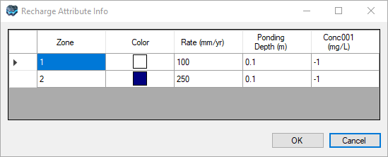
When the recharge zones were previously created, the values for the chemical species (Conc001) were left as undefined, indicated by -1. You will modify this for the smaller recharge area.
•Locate Zone2 (the second row in the table)
•Enter 5000 for Conc001 (replacing the -1 value).
•Click [OK] to close the Database window
•Now is a good time to save the project. Click [File]>[Save Project] from the main menu.
•Click [
![]()
] (Next Step) to proceed
•Select [Define Observations]
Define Concentration Observations
The final step before running the transport simulation is to add the three observation wells to the model to monitor the jet fuel concentrations at selected locations down-gradient of the refueling area. The first observation well (OW1) was installed immediately down-gradient of the refueling area shortly after the refueling operation started. The other two observation wells (OW2 and OW3) were installed two years later when elevated JP-4 concentrations were observed at the first well (OW1).
You will import the concentration observations from an Excel file.
•Click [File]>[Import Data] from the main menu bar
•Ensure 'Well' is selected as the Data Type
•[…] to choose the Source File.
•Browse to your Public 'My Documents' folder, then 'Visual MODFLOW Flex\Tutorials\Airport\suppfiles\Concentration_Observations.xlsx' file.
•[Open]
•[Next>>]
A preview window will appear displaying the source data.
•[Next>>]
•VMOD Flex provides you with various options to import well data.
•Choose the radio button [Well heads with the following data] radio button
•Then select [Observations points]
•Then select [Observed concentrations]

•Click [Next>>] to proceed to the Coordinate System step
•Click [Next>>] to accept the default Coordinate System and proceed to the Data Mapping step.
•In this screen, you need to map the fields from the spreadsheet to required fields in the Dells Import utility. To save time, you can prepare your Excel file with the exact filenames that are required by VMOD Flex, and then no mapping is required. For this exercise, the source Excel file has the map names pre-defined. Take a moment to review the required fields for the Wells import:
oWell Heads: Well ID, X/Y Coordinates, Elevation, and Well Bottom
oObservation Points: Logger Id, Logger Z, Concentration observation date, Observed concentration

•Click [Next>>] and the the Data Import preview will appear:

•[Finish]
The 'Concentration_Observations' will now appear as a new data object in the Data tree, as shown below.

Now you need to add these raw observation wells as observation points for the numerical model.
•Ensure that you are on the 'Define Observation' step in the numerical modeling workflow.
•Be sure that the 'Concentration_Observations' data object is selected in the tree
•Next, ensure that 'Well Observation' is selected from the first dropdown menu under the 'Toolbox' section.
•Click [Assign]>[Using Data Object] from the toolbox. Click on the [
![]()
] button to add the Well Observation object.
•A window will appear allowing you to select from available well groups, or to create a new well group:
•Select 'Create a new well group' and retain the default name.
•Ensure you have the options selected as shown below.
•Click [OK].

The observation wells ('Concentration Observations') will be added to the display and the numerical model tree, under NumericGrid1_r1/Run/Inputs/Observations.
•Locate 'Concentration Observations', and click on the box beside this data object in the Model Explorer
![]()
.

•You should now see several orange points in the model domain that represent the locations where head measurements were taken (if you don't, you may need to change the viewer to layer 1).

•Now is a good time to save the project. Click [File]>[Save Project] from the main menu.
•Click [
![]()
] (Next Step) to proceed.
•Select [Single Run], and click [
![]()
] (Next Step) to proceed
•At the 'Single Run' step, be sure to include MT3DMS in the engine run; place a check box
![]()
beside this engine in the list.
•Click [
![]()
] (Next Step) to proceed.
MT3DMS Translation Settings
This section will guide you through the selection of the advection method, solver settings, and output times that you will use to obtain the solution and results for the contaminant transport model.

Solution Method
•Expand the 'MT3DMS' item under the Translation settings, and select [Solution Method]. A Solution Method settings window will appear.
For this model run you will be using the Upstream Finite Difference solution method with the Implicit GCG Solver. The Upstream Finite Difference method provides a stable solution to the contaminant transport model in a relatively short period of time. The GCG solver uses an implicit approach to solving the finite difference equations, and is usually much faster than the explicit solution method.
•Click the button in the 'Advection Method' option and select [Upstream Finite Difference (UFD)]
•Click the button in the 'Use Implicit GCG Solver' option and select [Yes].
•The Implicit GCG Solver Settings window will appear in the lower half of the translation settings window, as shown in the image below:

Although the Upstream Finite Difference method and the Implicit GCG Solver are generally computationally efficient, the tutorial simulation tracks contaminant transport over a 20 year period. In order to speed up the modeling process, you will use a nonlinear time step. Type the following information in the fields at the bottom of the window.
•Maximum transport step size = 200, as in the image above
•Multiplier = 1.1
Output Control Settings
Next, you will define the output times at which you would like to see the contaminant transport modeling results.
•Under the 'MT3DMS' section in the Translation settings, select [Output Control]. The Translation settings will update as shown below.
•Enter 7305 for the 'Simulation time length'
•Enter 5000 for 'Max number of transport steps'
•The remaining defaults can be left as they were found, as shown in the image below:
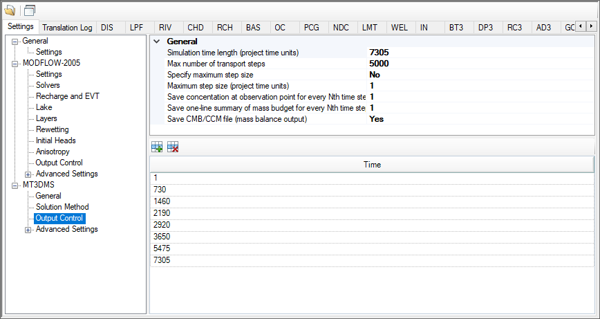
Output Times
•For this tutorial you will define specified times at which you would like to see the transport simulation results.
•The bottom half of the [Output Control] frame can be used to specify output times
•Click the [
![]()
] [Add Row] button; repeat this 7 more times.
•Enter the following output times in the grid.
MT3D Output times
| 1 |
| 730 |
| 1460 |
| 2190 |
| 2920 |
| 3650 |
| 5475 |
| 7305 |
•Now is a good time to save the project. Click [File]>[Save Project] from the main menu.
•You are now ready to translate the inputs into the MT3DMS packages.
•Click [
![]()
] to create the MODFLOW-2005 and MT3DMS packages. (this should take a few seconds)
•Click [
![]()
] (Next Step) to proceed.
Run MODFLOW-2005 and MT3DMS
In this step of the tutorial, you will run the flow and transport model:
•Click the [
![]()
] button to run MODFLOW-2005 and MT3DMS.
•The MODFLOW model run should complete in a few seconds; the MT3DMS run should also complete in under a minute.
•Once finished, you should see the message "***** The run was successful. *****" at the bottom of the engine progress window.

•In addition, you will see several items will be added to the model tree under 'Outputs': the 'Concentrations' was added to the model output tree under 'Output/Transport'.
•Now is a good time to save the project. Click [File]>[Save Project] from the main menu.
•Click [
![]()
] (Next Step) to proceed.
•Click [View Maps].
View Maps (Concentrations)
•By default, the Heads will be shown in the Maps view. In order to see the 'Concentrations', you need to turn off 'Heads' from the model explorer and turn on 'Concentrations'.
•Locate the 'Output' node on the model tree.
•Remove the Checkbox beside 'Heads'
•Add a checkbox beside 'Concentrations'
•In the viewer toolbar, activate the 'Cells' rendering option by clicking the [
![]()
] button and turn off the grid by clicking the [
![]()
]
button:
•The concentration results will be plotted for the first transport output time (in this case the first transport output time is 1 day). Note that, because the concentration color scale is automatically scaled to the largest values in any time step, the results from the first time step will appear all blue. As we will see shortly, we can change the color scale to match our needs. If you move your mouse around the viewer, you should see the calculated concentration change in the bottom right:
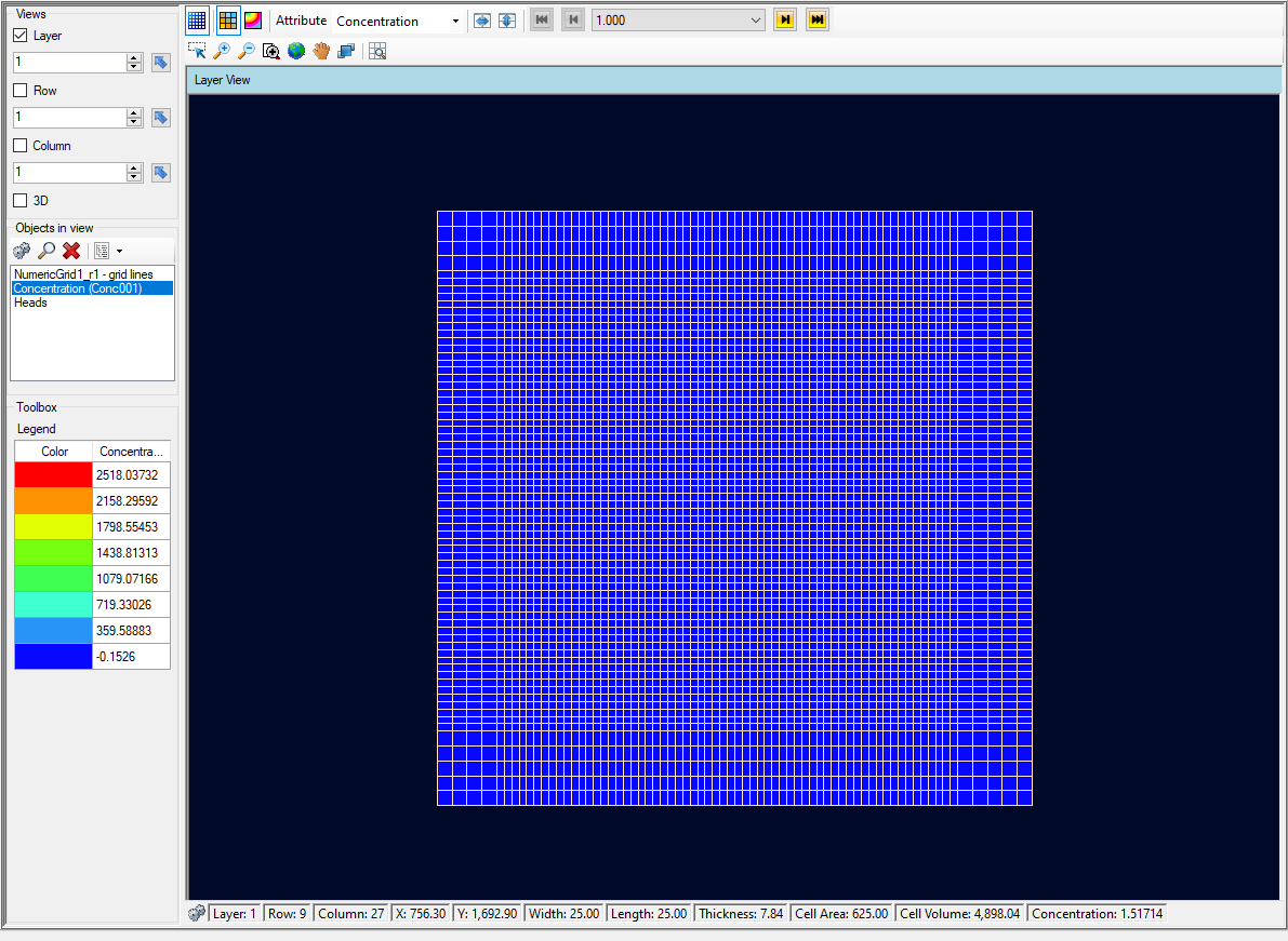
•In order to see the concentration results at the other output times, you need to advance the output time. Click on the time step buttons located on the toolbar above the 'Layer View', as shown below. Alternately, you can expand the list of output times, and navigate directly to the desired output time.
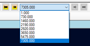
•The display will then update with a plot of concentration contours for the selected output time
•Open the last output time, day 7305, and the concentrations in the first layer of the model should look similar to the following figure:

Let's rescale the concentration results to a logarithmic scale, and apply a different color map.
•Right-click the Concentration (Conc001) output from the Model Explorer and select Settings...
•In the Settings menu, select Style > Colors to open up the color menu:
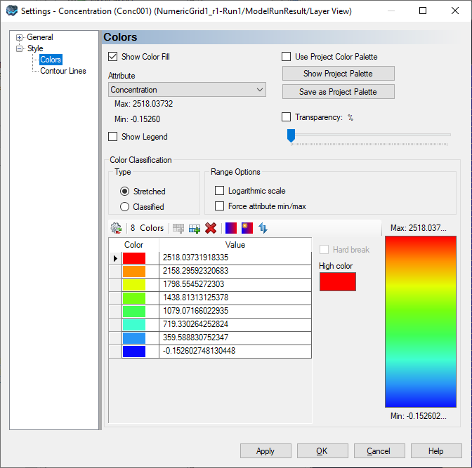
•Select the Assign colors from ramp (
![]()
) button and choose magma
•Select the Invert colors button(
![]()
), so that the high color is now black and the low color is white
•In the table, type 1000 for the first (highest) row, and 0.001 for the last (lowest) row. Check the box next to Logarithmic scale:

•Select OK. The final time step outputs in layer 1 should now look as follows (notice that the grid has been disabled for better visibility):
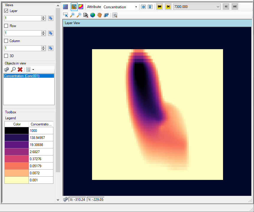
•Additionally, the outputs for layer 1 at 1.000 days look like the following:

View Charts (Concentrations)
In this section of the tutorial, you will learn how to compare the observed concentration data to the concentration values calculated by the model.
•Select [View Charts] item from the workflow tree.
•Click [Open Dashboard] to proceed.
•Click 'Chart selector' [
![]()
] button.
•Then, under 'Chart selector' check 'Time Series' and uncheck 'CalcVsObs'
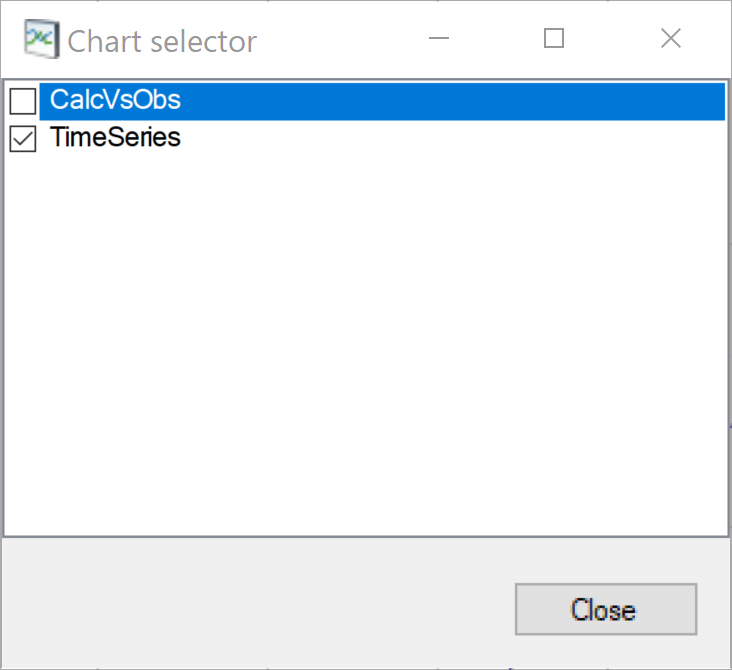
•Click [Close]
•Select the dropdown button in the first row of the table for the Species field and click [
![]()
] to select a filter from the Attribute Table. Note, you may wish to expand the table by clicking and dragging the separation line between the table and the chart to the right.
•Deselect all of the checkboxes except "Conc001" and click [OK].
You should now see the breakthrough curves for each of the three concentration observation wells defined earlier in the model (see following figure).

This time-series graph shows the calculated result using a colored line data series while the observation data is displayed only as data point symbols.
•Now is a good time to save the project. Click [File]>[Save Project] from the main menu.
*****This concludes the Airport Numerical Model with Transport tutorial*****


 59
59

 被折叠的 条评论
为什么被折叠?
被折叠的 条评论
为什么被折叠?
 到【灌水乐园】发言


