2.3 Airport Numerical Model with Transport

The following example walks through creating a numerical model with groundwater flow (using MODFLOW-2005) and basic contaminant transport (using MT3DMS). The exercise is based on the well-known Airport example from Visual MODFLOW Classic.

Objectives

•Learn how to create a project and create a numerical grid

•Become familiar with navigating the GUI and steps for numerical modeling

•Learn how to define new property zones and boundary conditions

•Define inputs for contaminant transport

•Translate the model inputs into MODFLOW and MT3DMS packages

•Run MODFLOW-2005 and MT3DMS engines

•Understand the results by interpreting heads, drawdown, and concentrations in several views

•Check the quality of the model by comparing observed heads to calculated heads, and observed vs. calculated concentrations

 Please Note: if you are unable to locate some supporting files for the tutorial, you may download these from the website.

Create the Project

•Launch Visual MODFLOW Flex.

•Select [File] then [New Project..]. The Create Project dialog will appear.

•Type in project name 'Airport Tutorial'.

•Click the [

] button, and navigate to a folder where you wish your projects to be saved, and click [OK].

•Define your coordinate system and datum (or just leave the Local Cartesian as defaults).

For this project, the default units will be fine. The Create Project dialog should look similar to the following:

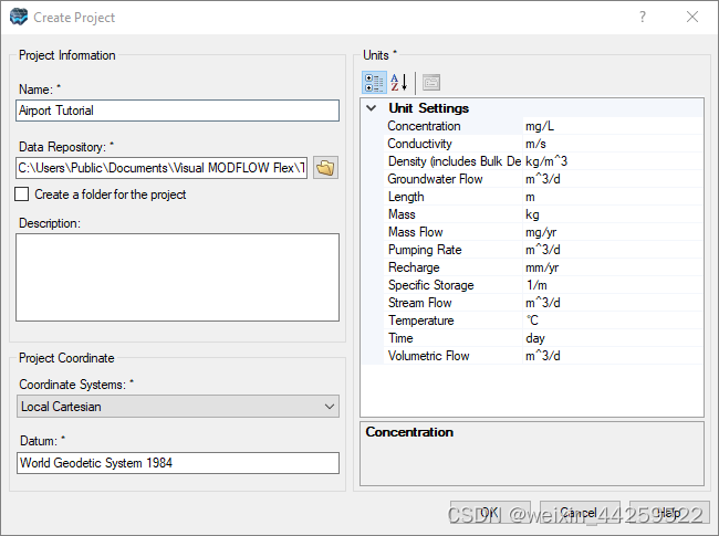
•Click [OK].  The workflow selection screen will appear.

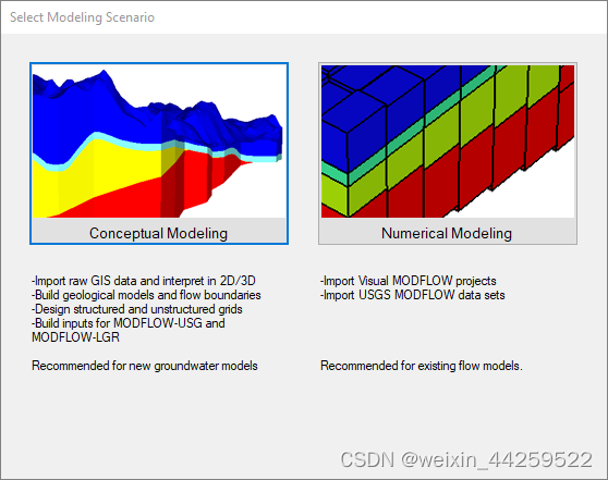
•Select [Numerical Modeling] and the Numerical Modeling workflow will load.  

•The first step is to Define Modeling Objectives.

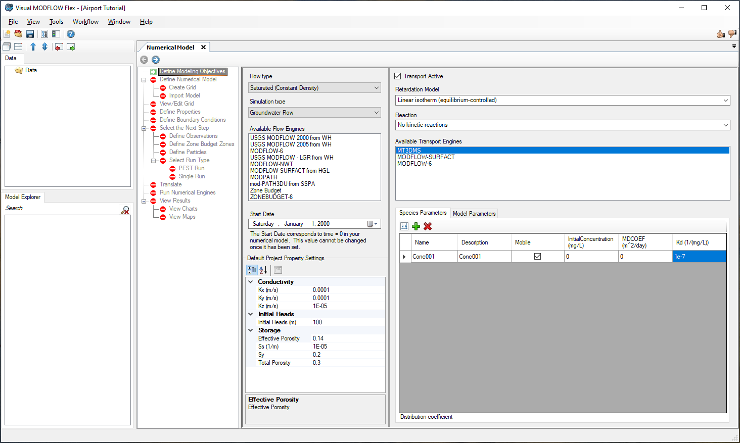
Define Modeling Objectives

•In this step, you define the objectives of your model and the default parameters.

•The Start Date of the model corresponds to the beginning of the simulation time period.

•Select 1/1/2000 for the Start Date

•For this scenario, we will include contaminant transport in the model run. Click the check box beside 'Transport Active' (in the right hand side of the window, under Define Modeling Objectives.

•For 'Retardation Model' select 'Linear isotherm (equilibrium-controlled)'. For this tutorial you will not be simulating any decay or degradation of the contaminant, so the default 'Reaction' setting of 'No kinetic reactions' will be fine.

•Below the 'Retardation Model' and 'Reaction' settings are two tabs: 'Species Parameters' and 'Model Parameters'. By default, one species (chemical component) is defined for the transport run. For this example, we will leave the initial concentration ('InitialConcentration (mg/L)') as zero, but adjust Kd (the distribution coefficient)

•Type 1E-7 in [Kd 1/(mg/L)] column

•You are now finished setting up the flow and transport objectives. Click [

] (Next Step) to proceed.

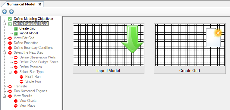
•The following 'Define Numerical Model' step will appear; at this step, you can import Visual MODFLOW Classic or MODFLOW data sets, or define a new empty grid. For this tutorial we will create a new grid.

•Click on [Create Grid] to proceed

Create Grid

•At this step, you can specify the dimensions of the Model Domain, and define the number of rows, columns, and layers for the finite difference grid. Type the following into the Grid Size section,

•Columns: 40

•Rows: 40

•For Grid Extents, enter 2000 for Xmax and 2000 for Ymax

•Under Define Vertical Grid, Type 3 for Number of Layers

Define Layer Elevations

•In Visual MODFLOW Flex, you can define the elevations of the tops and bottom of the model layers. Or you can have varying layer elevations defined from Surface data objects.  Surfaces could be from data objects you imported from Surfer (.GRD, ESRI .ASI, .DEM), or from Surfaces you have created through interpolating XYZ points.  In this exercise, you will import 4 surfaces (from Surfer .GRD files), then use these to define the layer elevations.

•Click [File] then [Import Data...] from the main menu. The following window will appear:

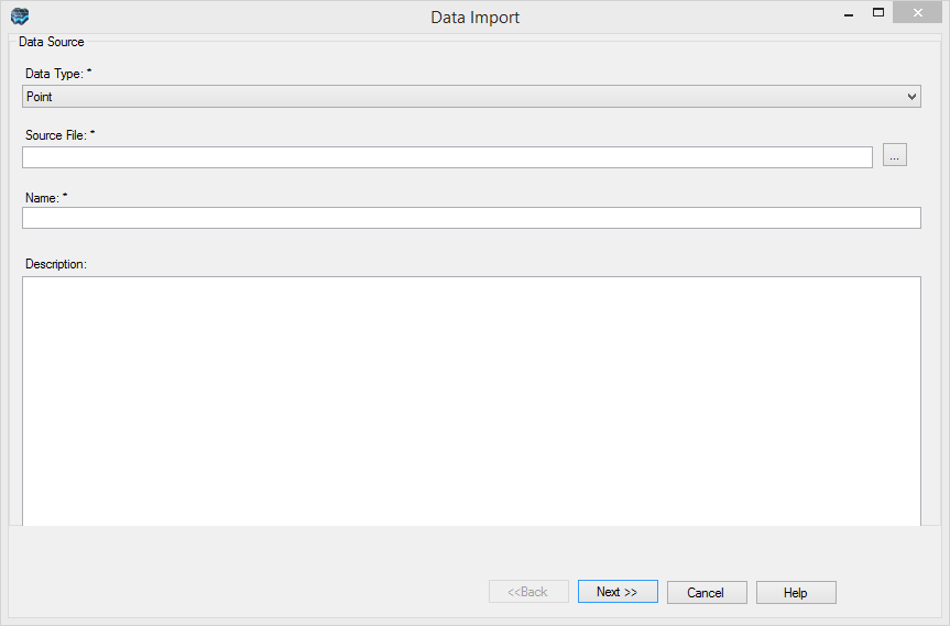
•For the Data Type, select 'Surface' from the drop-down list.

•In the Source File field click the […] button and navigate to your Public "My Documents" folder, then "Visual MODFLOW Flex\Tutorials\Airport\suppfiles\Surfer\airport-ground-surface.grd"  and select [Open]

•Click [Next>>]

•Click [Next>>] (accept the defaults)

•Click [Next>>] (accept the defaults)

•Click [Finish].  You should now see a new "airport-ground-surface" data object appear in the data tree, in the top left corner of the window.

•Now, repeat the above steps to import the other Surfer .GRD files into the project:  

oairport-layer2-top.grd

oairport-layer3-top.grd

oairport-layer3-bottom.grd

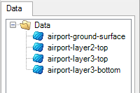
•When you are finished, you should see 4 Surface data objects in the data tree in the top left corner.  

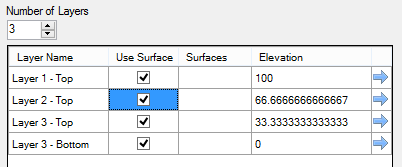
•Now you are ready to define the grid layers using these surfaces.  Under Number of Layers, select 'Use Surface' check box for each grid layer.  This is shown below

•Next you will provide a surface for each layer;

•Click on airport-ground-surface from the data object tree (it should become selected), then click on the topmost blue arrow [

] beside 'Use Surface' in the Number of Layers table (in the row that starts "Layer 1 - Top".   If you have done this correctly, the table should appear as shown below.
 

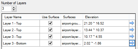
•Now repeat these steps for the remaining layers:

•Select airport-layer2-top Surface data object to the tree, and insert this (using the [

]) as the Surface for Layer 2 - Top

•Select airport-layer3-top Surface data object to the tree, and insert this (using the [

]) as the Surface for Layer 3 - Top

•Select airport-layer3-bottom Surface data object to the tree, and insert this (using the [

]) as the Surface for Layer 3 - Bottom

•When you are finished, the table should appear as shown below.
 

•You are finished defining the layer elevations.  

•Click on the [Create Grid] button (near the top right of the window) to create the grid. You will see the model tree will be generated on the left side of the window, and 'NumericGrid1' should appear as the last item.

Refine the Grid

This section describes the steps necessary to refine the model grid in areas of interest, such as around the water supply wells, refueling area, and area of discontinuous aquitard. The reason for refining the grid is to get more detailed simulation results in areas of interest, or in zones where you anticipate steep hydraulic gradients. For example, if drawdown is occurring around the well, the water table will have a smoother surface if you use a finer grid spacing. Also, layer properties can be assigned more correctly on a finer grid.

•Right click on the 'NumericalGrid1' from the tree, and select [Edit Numerical Grid...]

•The following window will appear:

The grid refinement works by defining a starting row number, and ending row number, then a 'Refine by' factor; to help you define the limits of where the refinement should be applied, you can add data objects to this display, such as well locations, arial maps, shapefiles, etc.  When you are using this feature with your own models, you will need to import these data object files before starting the 'Grid Refinement' step.

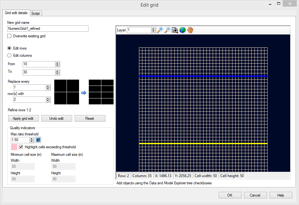
•You will first start by refining the rows.

•Enter '5' in the 'From' field, and enter '35' in the 'To' field.

•Enter 'Replace Every [1] row(s) with [2]'.  Your screen should appear as follows:

 

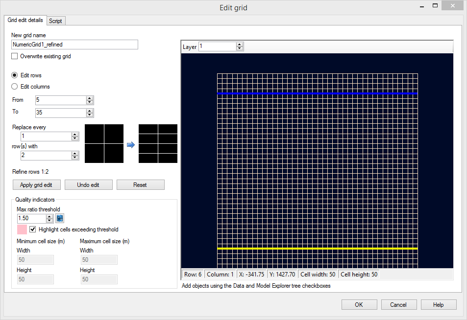
•Click on the [Apply grid edit] button.

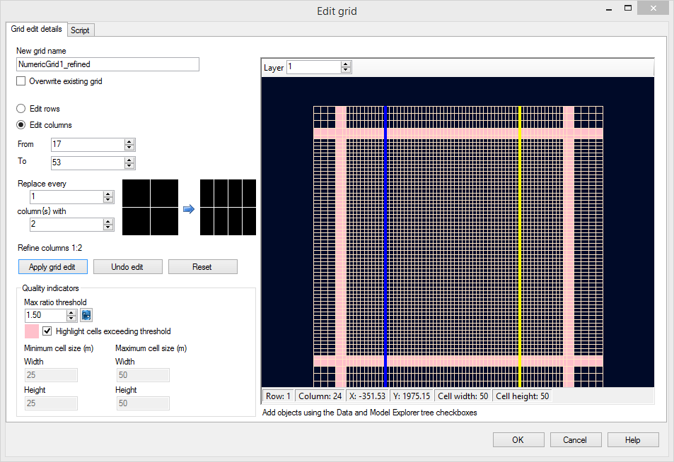
•Next, you will refine the columns.

•At the top left of the window, select the [Edit Columns] radio button.

•As before, Enter '5' in the 'From' field, and enter '35' in the 'To' field.

•Enter Replace every [1] column(s) with [2]

•Click on the [Apply grid edit] button.

You should now see coarse grid sizes around the edge of the model domain, and a more finer sized grid spacing in the middle of model (around the areas interest). This is shown below. The band of pink cells around the edges of the refinement indicate cells where the Max ratio threshold quality indicator (which is set by default to a cell step size of 1.50) has been exceeded. This can sometimes result in larger computational times and the potential for increased grid based dispersion. These areas can be further fractionally refined to improve the grid quality; in this exercise, we will leave the grid as-is and proceed to the next step.

•Click on the [OK] button.

In the Model Explorer tree, a new grid and numeric workflow (i.e. 'NumericGrid1_refined') is created, and a new workflow window/tab (i.e. 'NumericGrid1_refined-Run1') opens.  At this stage we will continue working with the refined grid, and we can ignore the initial coarse grid.

•In the next section, you will view the numerical grid that you just created.

•Click on the Define Properties step or click the next button [

] to proceed.

Define Flow Properties

This section will guide you through the steps necessary to design a model with layers of highly contrasting hydraulic conductivities.

•First, ensure that 'Conductivity' is selected in the first dropdown menu under the 'Toolbox'

•Click on the [Edit...] button and Type the following values in the top row of the window:

oKx (m/s): 2E-4, then use [F2] to propagate through all cells

oKy (m/s): 2E-4, then use [F2] to propagate through all cells

oKz (m/s): 2E-4, then use [F2] to propagate through all cells

•Click [OK] to accept these values.
 
 

 Please Note:  it may take a moment for Flex to process this change.
 

In this case the Kx, Ky, and Kz values are the same, indicating the assigned property values are assumed horizontally and vertically isotropic. However, anisotropic property values can be assigned to a model by modifying the Conductivity Database.

In this three layer model:

•Layer 1 represents the upper aquifer

•Layer 2 represents the aquitard separating the upper and lower aquifers, and

•Layer 3 represents the lower aquifer.

For this example, we will use the previously assigned hydraulic conductivity values (Zone# 1) for model layers 1 and 3 (representing the aquifers) and assign different Conductivity values (i.e. a new Zone) for model layer 2 (representing the aquitard). Note that layer 1 is the top model layer.

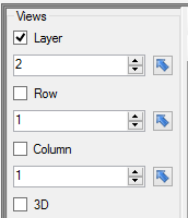
•Next you need to change to Layer 2. (using the up arrow under the Layer text box shown below)

You are now viewing the second model layer, representing the aquitard. The next step in this tutorial is to assign a lower hydraulic conductivity value to the aquitard (layer 2). We can graphically assign the property values to the model grid cells.

•Click [Assign] then [Entire Layer/Row/Column] from the toolbox.

The following dialog will appear:

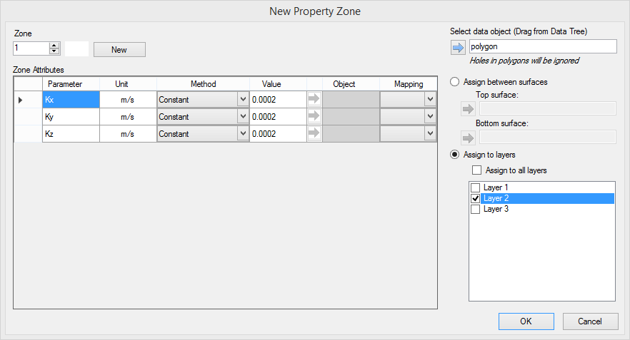
•Click on the [New] button at the top; this will create a new zone.

•Enter the following values:

oKx (m/s): 1E-10

oKy (m/s): 1E-10

oKz (m/s): 1E-11

The dialog should appear as shown below:

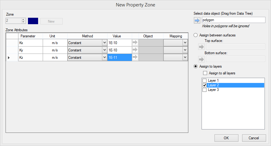
• Click [OK] to accept these values.

Once finished, the cells for Layer2 should change blue, which indicates these cells belong to Zone2; you can use the Legend under the toolbox as a guide, and also mouse over cells in the grid view, and note the values in the status bar.

 

Next you must assign the appropriate conductivity values to the discontinuous region. Although the region where the aquitard pinches out is very thin, the conductivity values of these grid cells should be set equal to the Conductivity values of either the upper or lower aquifers.In this particular example, the zone of discontinuous aquitard is indicated on a shapefile. We will import this shapefile into the project:

•Click [File] then [Import data...]

•For the Data Type, select Polygon from the drop-down list.

•In the Source File field click the […] button and navigate to your Public "My Documents" folder, then 'VMODFlex\Tutorials\Airport\suppfiles\discontinuous-aquitard.shp', and click [Open]

•Click [Next>>]

•Click [Next>>] (accept the defaults)

•Click [Next>>] (accept the defaults)

•Click [Finish].  

•You should now see a new data object, 'discontinuous-aquitard' appear in the data