U-net模型的实现和完整代码

carrot！。

已于 2023-04-30 17:04:35 修改

阅读量3k

点赞数 1

分类专栏： U-net图像分割文章标签： pytorch 图像处理计算机视觉

于 2023-04-30 17:03:44 首次发布

本文链接：https://blog.csdn.net/weixin_44532482/article/details/130449242

版权

U-net图像分割专栏收录该内容

1 篇文章

订阅专栏

U-net是非常经典的图像分割模型，在整个结构中没有全连接层，使用上采样层代替。详细的可以阅读U-net的原论文详细了解，原文链接：https://arxiv.org/pdf/1505.04597.pdf

同时在网上也有许多优秀的文章、博客做出了非常好的解读大家可以搜索查看。

代码主要分为数据的预处理、网络结构的搭建、训练、测试下面是详细的代码

1、数据的预处理代码保存在datesetpretrain.py文件中，本人是参考了https://blog.csdn.net/qq_44886601/article/details/127886731这篇文章大家可以去看一下，作者也做出了详尽的讲解

import os
from torch.utils.data import Dataset
from torchvision import transforms
from PIL import Image
import matplotlib.pyplot as plt
transform = transforms.Compose([
    transforms.Resize((572, 572)),  # 缩放图像与原论中输入图像大小一致
    transforms.ToTensor(),  
])


# 数据处理文件
class Data_Loader(Dataset):  # 加载数据
    def __init__(self, root, transforms=transform):  # 指定路径、预处理等等
        imgs = os.listdir(root)  # 获取root文件下的文件
        self.imgs = [os.path.join(root, img) for img in imgs]  # 获取每个文件的路径
        self.transforms = transforms  # 预处理

    def __getitdem__(self, index):  # 读取图片，返回一条样本
        image_path = self.imgs[index]  # 根据index读取图片
        label_path = image_path.replace('image', 'label')  # 把路径中的image替换成label，就找到对应数据的label

        image = Image.open(image_path)  # 读取图片和对应的label图
        label = Image.open(label_path)

        if self.transforms:  # 判断是否预处理
            image = self.transforms(image)

            label = self.transforms(label)
            label[label >= 0.5] = 1  # 这里转为二值图片
            label[label < 0.5] = 0

        return image, label

    def __len__(self):  # 返回图像个数
        return len(self.imgs)

2、U-net结构搭建与训练。我这个把网络的搭建与训练写到一个文件中了，这点可能做的不好，我也看了许多作者都是分开写的，我当时就是图方便。在网络结构是参考https://blog.csdn.net/weixin_41857483/article/details/120768804同样，也是非常详细的介绍了网络结构，代码如下：

import torch.nn as nn
import torch.nn.functional as F
import torch
import torch.optim as optim
import datesetpretrain #导入数据预处理的部分

class DoubleConv(nn.Module):
    """
    1. DoubleConv 模块
    (convolution => [BN] => ReLU) * 2
    连续两次的卷积操作：U-net网络中，下采样和上采样过程，每一层都会连续进行两次卷积操作
    """
    def __init__(self, in_channels, out_channels):
        super().__init__()
        # torch.nn.Sequential是一个时序容器，Modules 会以它们传入的顺序被添加到容器中。
        # 此处：卷积->BN->ReLU->卷积->BN->ReLU
        self.double_conv = nn.Sequential(
            nn.Conv2d(in_channels, out_channels, kernel_size=3, padding=0),
            nn.BatchNorm2d(out_channels),
            nn.ReLU(inplace=True),
            nn.Conv2d(out_channels, out_channels, kernel_size=3, padding=0),
            nn.BatchNorm2d(out_channels),
            nn.ReLU(inplace=True)
        )

    def forward(self, x):
        return self.double_conv(x)


class Down(nn.Module):
    """
    2. Down(下采样)模块
    Downscaling with maxpool then double conv
    maxpool池化层，进行下采样，再接DoubleConv模块
    """
    def __init__(self, in_channels, out_channels):
        super().__init__()
        self.maxpool_conv = nn.Sequential(
            nn.MaxPool2d(2),  # 池化层
            DoubleConv(in_channels, out_channels)  # DoubleConv模块
        )

    def forward(self, x):
        return self.maxpool_conv(x)


class Up(nn.Module):
    """
    3. Up(上采样)模块
    Upscaling then double conv
    """
    """
      __init__初始化函数定义了上采样方法以及卷积采用DoubleConv
      上采样，定义了两种方法：Upsample和ConvTranspose2d，也就是双线性插值和反卷积。
    """
    def __init__(self, in_channels, out_channels, bilinear=True):
        super().__init__()

        # if bilinear, use the normal convolutions to reduce the number of channels
        if bilinear:
            self.up = nn.Upsample(scale_factor=2, mode='bilinear', align_corners=True)
        else:
            self.up = nn.ConvTranspose2d(in_channels, in_channels // 2, kernel_size=2, stride=2)  # 反卷积(2*2 => 4*4)

        self.conv = DoubleConv(in_channels, out_channels)

    def forward(self, x1, x2):
        """
        x1接收的是上采样的数据，x2接收的是特征融合的数据
        特征融合方法就是，先对小的feature map进行padding，再进行concat(通道叠加)
        :param x1:
        :param x2:
        :return:
        """
        x1 = self.up(x1)
        # input is CHW
        diffY = x2.size()[2] - x1.size()[2]
        diffX = x2.size()[3] - x1.size()[3]

        x1 = F.pad(x1, [diffX // 2, diffX - diffX // 2,
                        diffY // 2, diffY - diffY // 2])
        print(diffX - diffX // 2)
        x = torch.cat([x2, x1], dim=1)
        return self.conv(x)


class OutConv(nn.Module):
    """
    4. OutConv模块
    UNet网络的输出需要根据分割数量，整合输出通道(若最后的通道为2，即分类为2的情况)
    """
    def __init__(self, in_channels, out_channels):
        super(OutConv, self).__init__()
        self.conv = nn.Conv2d(in_channels, out_channels, kernel_size=1)

    def forward(self, x):
        return self.conv(x)


"""
UNet网络用到的模块即以上4个模块
根据UNet网络结构，设置每个模块的输入输出通道个数以及调用顺序
"""


class UNet(nn.Module):
    def __init__(self, n_channels, n_classes, bilinear = False):
        super(UNet, self).__init__()
        self.n_channels = n_channels
        self.n_classes = n_classes
        self.bilinear = bilinear

        self.inc = DoubleConv(n_channels, 64)
        self.down1 = Down(64, 128)
        self.down2 = Down(128, 256)
        self.down3 = Down(256, 512)
        self.down4 = Down(512, 1024)
        self.up1 = Up(1024, 512, bilinear)
        self.up2 = Up(512, 256, bilinear)
        self.up3 = Up(256, 128, bilinear)
        self.up4 = Up(128, 64, bilinear)
        self.outc = OutConv(64, n_classes)
    def _initialize_weights(self):
        for module in self.modules():
            if isinstance(module, nn.Conv2d) or isinstance(module, nn.Linear):
                nn.init.kaiming_normal_(module.weight)
                if module.bias is not None:
                    module.bias.data.zero_()
            elif isinstance(module, nn.BatchNorm2d):
                module.weight.data.fill_(1)
                module.bias.data.zero_()

    def forward(self, x):
        x1 = self.inc(x)
        x2 = self.down1(x1)
        x3 = self.down2(x2)
        x4 = self.down3(x3)
        x5 = self.down4(x4)
        x = self.up1(x5, x4)
        x = self.up2(x, x3)
        x = self.up3(x, x2)
        x = self.up4(x, x1)
        logits = self.outc(x)
        return logits

#下面是训练的部分
'''if __name__ == '__main__':
    net = UNet(n_channels=1, n_classes=1)
    trainset=datesetpretrain.Data_Loader("./data/train/image")
    train_loader = torch.utils.data.DataLoader(dataset=trainset,batch_size=4,shuffle=True)
    optimizer=optim.RMSprop(net.parameters(),lr=0.00001,weight_decay=1e-8,momentum=0.9)
    criterion=nn.BCEWithLogitsLoss()

    save_path = './UNet.pth'
    print(net)
    for epoch in range(20):

        net.train()  # 训练模式
        running_loss = 0.0

        for image, label in train_loader:  # 读取数据和label
            #print(image.shape)
            #print(label.shape)
            optimizer.zero_grad()  # 梯度清零
            pred = net(image)  # 前向传播
            pred=F.pad(pred,[4,4,4,4])
            #print(pred.shape)
            #print(label.shape)在这里我遇到了问题在下文解释
            loss = criterion(pred, label)  # 计算损失
            loss.backward()  # 反向传播
            optimizer.step()  # 梯度下降
            running_loss += loss.item()  # 计算损失和

            print("train_loss:%0.3f" % (loss.item()))

    torch.save(net.state_dict(), save_path)'''

在代码中我做出了标记就是在倒数第9行的位置，我输出了一下pred与label的形状，pred的做完向前传播的矩阵是[4,1,564,564]，而我们在输入的时候是572*572的图像大小经过向前传播却变小了，我估计是在网络结构中出现了问题，本人目前还不清楚蛋初步估计是在上采样中出现了问题也就是在


    def forward(self, x1, x2):
        """
        x1接收的是上采样的数据，x2接收的是特征融合的数据
        特征融合方法就是，先对小的feature map进行padding，再进行concat(通道叠加)
        :param x1:
        :param x2:
        :return:
        """
        x1 = self.up(x1)
        # input is CHW
        diffY = x2.size()[2] - x1.size()[2]
        diffX = x2.size()[3] - x1.size()[3]

        x1 = F.pad(x1, [diffX // 2, diffX - diffX // 2,
                        diffY // 2, diffY - diffY // 2])
        print(diffX - diffX // 2)
        x = torch.cat([x2, x1], dim=1)
        return self.conv(x)

F.pad()中，这是我的猜想。于是我在向前传播完成后对生成的pred结果使用了补上了4圈0的办法解决了问题，因为在计算损失函数时需要pred与label的形状相同。训练完成将数据保存在UNet.pth文件中

3、效果测试，参考文件如下

import numpy as np
import torch
from torchvision import transforms
from PIL import Image
import Unet
import matplotlib.pyplot as plt

transform = transforms.Compose([
    transforms.ToTensor(),
    transforms.Normalize((0.5,), (0.5))
])#对测试集的图像做预处理

# 加载模型和在UNet.pth中的参数
device = torch.device('cuda' if torch.cuda.is_available() else 'cpu')
net = Unet.UNet(n_channels=1, n_classes=1)
net.load_state_dict(torch.load('UNet.pth', map_location=device))
net.to(device)

net.eval()
with torch.no_grad():
    img = Image.open('./data/test/1.png')  # 读取预测的图片
    img = transform(img)  # 预处理
    img = torch.unsqueeze(img, dim=0)
    pred = net(img.to(device))  # 网络预测
    pred = torch.squeeze(pred)  # 将(batch、channel)维度去掉
    pred = np.array(pred.data.cpu())  # 保存图片需要转为cpu处理
    pred[pred >= 0] = 255  # 转为二值图片
    pred[pred < 0] = 0
    pred = np.uint8(pred)  # 转为图片的形式
    plt.imshow(pred)
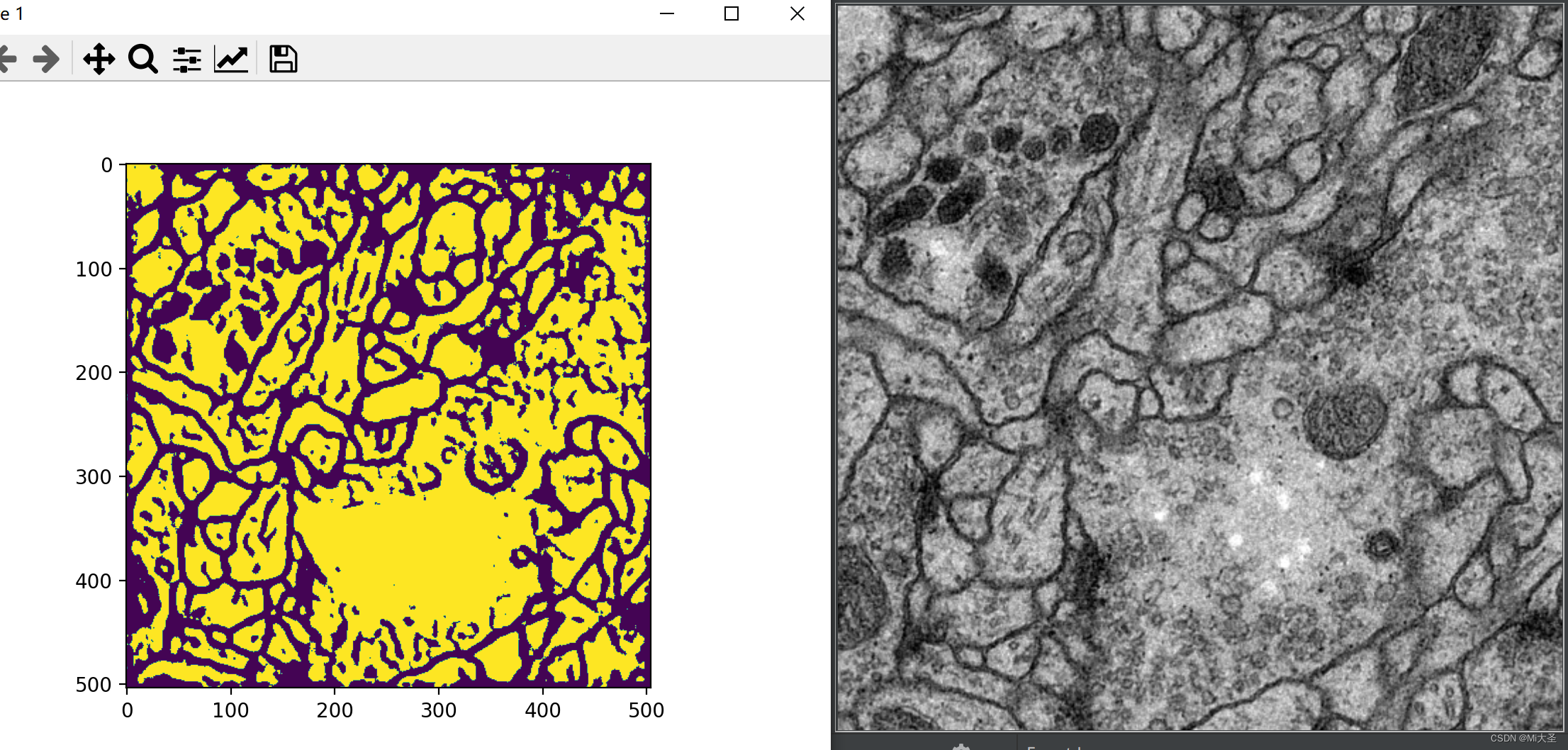
    plt.show()

最后是结果对比个人感觉还不错，只是我没有做精度的测算，对比图如下：