模型量化（二）—— 训练后量化PTQ（全代码）

训练后量化（Post-training Quantization，PTQ）是一种常见的模型量化技术，它在模型训练完成之后应用，旨在减少模型的大小和提高推理速度，同时尽量保持模型的性能。训练后量化对于部署到资源受限的设备上，如移动设备和嵌入式设备，特别有用。

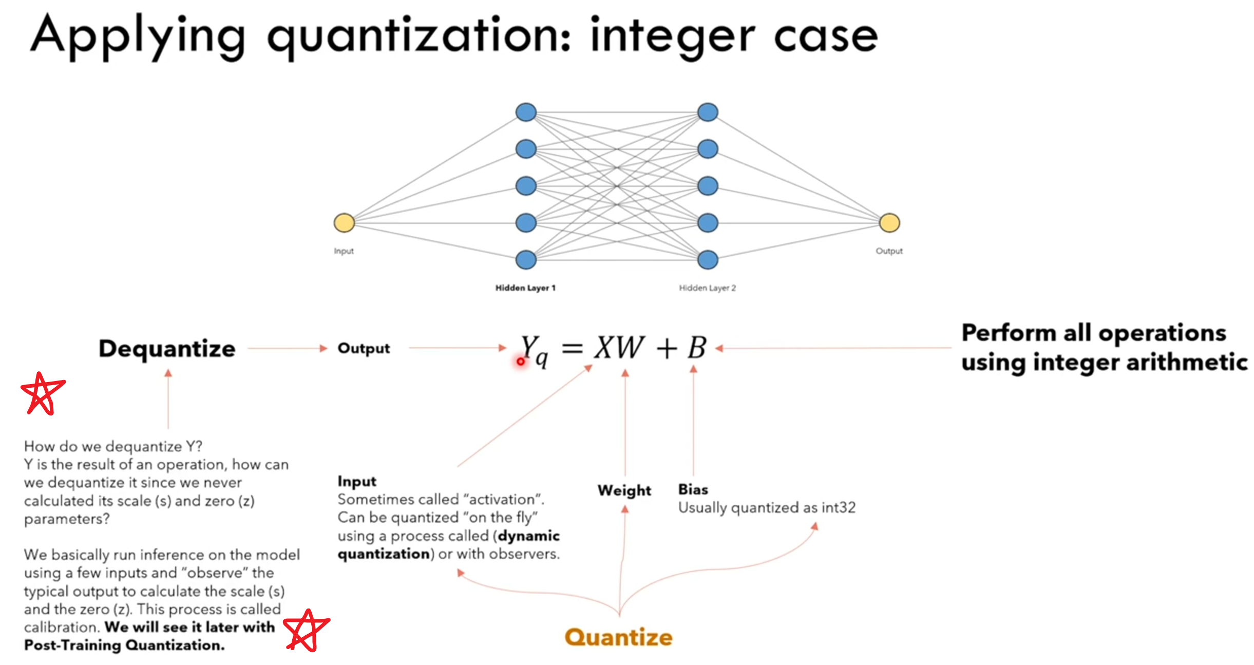
在我们量化时，量化操作可以应用于模型的输入、权重 和 激活（即神经元输出值）上。

但我们发现，对于激活值，我们执行反量化时，并不知道这些激活值对应的浮点数矩阵的最大值和最小值，即我们执行非对称或对称量化里面的 𝛼, β 参数，所以我们拿到一个模型时，最多只能对它的权重W和输入X做量化，对于激活值Y的反量化，我们需要一组小的calibration set数据来初步计算对于Y的S和Z参数。

不熟悉非对称或对称量化的朋友可以康康这篇：《模型量化（一）—— 非对称量化、对称量化（全代码）》

 

 

PTQ流程：

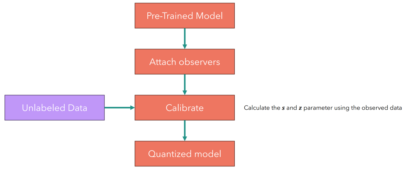
Observer，顾名思义就是模型在正常inference的时候会被记录下正常的浮点激活值，用来算激活值对应的S和Z参数。

Calibrate后模型的W和Y都有对应的S和Z了，模型名义上量化完成。浮点的输入X也能off-line地实时算它对应的S和Z。

所以量化后的模型运行时，先对浮点输入进行量化，然后与整型的W矩阵相乘，得到整型的激活值，这时再反量化为浮点激活值，对应于下一个神经元的浮点输入，依次循环。
大家可能会想吗，这么麻烦，又是量化又是反量化，怎么还会压缩模型和加速模型呢？

压缩模型：原本所有的W都是浮点数存储，比如float32，现在转换为int8存储，模型尺寸减了大概4倍；再额外存一些神经元或网络层的S和Z参数（取决于量化的粗粒度），相对于W来说占内存很小（如果是很细粒度的量化可能这部分也得好好考虑，量化的粒度分为权重级量化、层级量化、通道级量化等）。

加速模型：主要的收益是使得模型中占大头的 W * X 操作变成了整型相乘，功耗和时延最低（浮点数相乘时功耗和时延最大）。3 * 100 * 100 * 10的全连接网络中，有213个神经元，但是有 3 * 100 * 100 * 10 = 300M个参数！这还是忽略了bias。量化相当于就是让这 300M 次乘法更轻量。而相对的 overhead 就是对开头的3 + 100 + 100 = 203个中间输入进行一下量化 和 对 100 + 100 + 10 = 210个激活值进行一下反量化，这部分开销随着网络层数与参数的增加几乎可以忽略不计。
一些专门的深度学习加速器和现代CPU/GPU提供了对低位宽整数（如int8）的优化支持，用这些硬件后可以更加体现模型量化的优势。

量化会带来一定的量化误差，即模型精度会受影响，这肯定的，但按经验来说几乎没什么影响，不要压到int4或int2这么极限就行。

 

全代码

预训练模型

import torch
import torchvision.datasets as datasets 
import torchvision.transforms as transforms
import torch.nn as nn
import matplotlib.pyplot as plt
from tqdm import tqdm
from pathlib import Path
import os

# Make torch deterministic
_ = torch.manual_seed(0)

transform = transforms.Compose([transforms.ToTensor(), transforms.Normalize((0.1307,), (0.3081,))])

# Load the MNIST dataset
mnist_trainset = datasets.MNIST(root='./data', train=True, download=True, transform=transform)
# Create a dataloader for the training
train_loader = torch.utils.data.DataLoader(mnist_trainset, batch_size=10, shuffle=True)

# Load the MNIST test set
mnist_testset = datasets.MNIST(root='./data', train=False, download=True, transform=transform)
test_loader = torch.utils.data.DataLoader(mnist_testset, batch_size=10, shuffle=True)

# Define the device
device = "cpu"


# Define the model
class VerySimpleNet(nn.Module):
    def __init__(self, hidden_size_1=100, hidden_size_2=100):
        super(VerySimpleNet,self).__init__()
        self.linear1 = nn.Linear(28*28, hidden_size_1) 
        self.linear2 = nn.Linear(hidden_size_1, hidden_size_2) 
        self.linear3 = nn.Linear(hidden_size_2, 10)
        self.relu = nn.ReLU()

    def forward(self, img):
        x = img.view(-1, 28*28)
        x = self.relu(self.linear1(x))
        x = self.relu(self.linear2(x))
        x = self.linear3(x)
        return x

net = VerySimpleNet().to(device)


# Train the model
def train(train_loader, net, epochs=5, total_iterations_limit=None):
    cross_el = nn.CrossEntropyLoss()
    optimizer = torch.optim.Adam(net.parameters(), lr=0.001)

    total_iterations = 0

    for epoch in range(epochs):
        net.train()

        loss_sum = 0
        num_iterations = 0

        data_iterator = tqdm(train_loader, desc=f'Epoch {epoch+1}')
        if total_iterations_limit is not None:
            data_iterator.total = total_iterations_limit
        for data in data_iterator:
            num_iterations += 1
            total_iterations += 1
            x, y = data
            x = x.to(device)
            y = y.to(device)
            optimizer.zero_grad()
            output = net(x.view(-1, 28*28))
            loss = cross_el(output, y)
            loss_sum += loss.item()
            avg_loss = loss_sum / num_iterations
            data_iterator.set_postfix(loss=avg_loss)
            loss.backward()
            optimizer.step()

            if total_iterations_limit is not None and total_iterations >= total_iterations_limit:
                return
            
def print_size_of_model(model):
    torch.save(model.state_dict(), "temp_delme.p")
    print('Size (KB):', os.path.getsize("temp_delme.p")/1e3)
    os.remove('temp_delme.p')

MODEL_FILENAME = 'simplenet_ptq.pt'

if Path(MODEL_FILENAME).exists():
    net.load_state_dict(torch.load(MODEL_FILENAME))
    print('Loaded model from disk')
else:
    train(train_loader, net, epochs=1)
    # Save the model to disk
    torch.save(net.state_dict(), MODEL_FILENAME)


# Define the testing loop
def test(model: nn.Module, total_iterations: int = None):
    correct = 0
    total = 0
    iterations = 0

    model.eval()

    with torch.no_grad():
        for data in tqdm(test_loader, desc='Testing'):
            x, y = data
            x = x.to(device)
            y = y.to(device)
            output = model(x.view(-1, 784))
            for idx, i in enumerate(output):
                if torch.argmax(i) == y[idx]:
                    correct +=1
                total +=1
            iterations += 1
            if total_iterations is not None and iterations >= total_iterations:
                break
    print(f'Accuracy: {round(correct/total, 3)}')


# Print weights and size of the model before quantization

# Print the weights matrix of the model before quantization
print('Weights before quantization')
print(net.linear1.weight)
print(net.linear1.weight.dtype)

print('Size of the model before quantization')
print_size_of_model(net)

print(f'Accuracy of the model before quantization: ')
test(net)

加入Observer

# Insert min-max observers in the model

class QuantizedVerySimpleNet(nn.Module):
    def __init__(self, hidden_size_1=100, hidden_size_2=100):
        super(QuantizedVerySimpleNet,self).__init__()
        self.quant = torch.quantization.QuantStub()
        self.linear1 = nn.Linear(28*28, hidden_size_1) 
        self.linear2 = nn.Linear(hidden_size_1, hidden_size_2) 
        self.linear3 = nn.Linear(hidden_size_2, 10)
        self.relu = nn.ReLU()
        self.dequant = torch.quantization.DeQuantStub()

    def forward(self, img):
        x = img.view(-1, 28*28)
        x = self.quant(x)
        x = self.relu(self.linear1(x))
        x = self.relu(self.linear2(x))
        x = self.linear3(x)
        x = self.dequant(x)
        return x

net_quantized = QuantizedVerySimpleNet().to(device)
# Copy weights from unquantized model
net_quantized.load_state_dict(net.state_dict())
net_quantized.eval()

net_quantized.qconfig = torch.ao.quantization.default_qconfig
net_quantized = torch.ao.quantization.prepare(net_quantized) # Insert observers
net_quantized

校准模型

#用测试集再跑一次装了observer的模型
test(net_quantized)

print(f'Check statistics of the various layers')
net_quantized

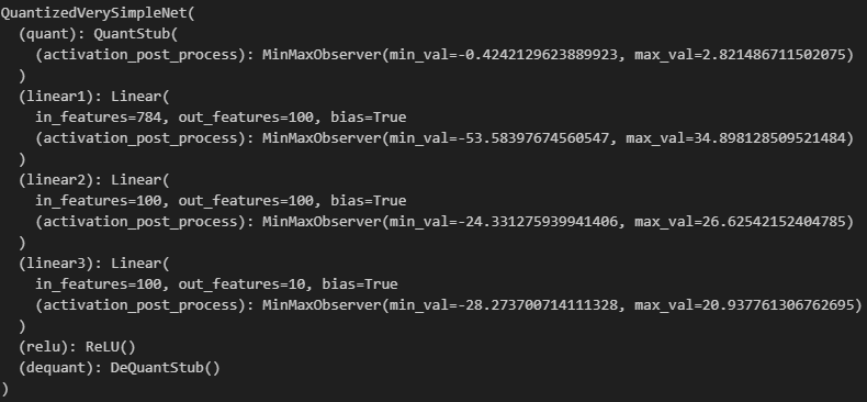
这时看到激活层的 𝛼, β 都有了，good！

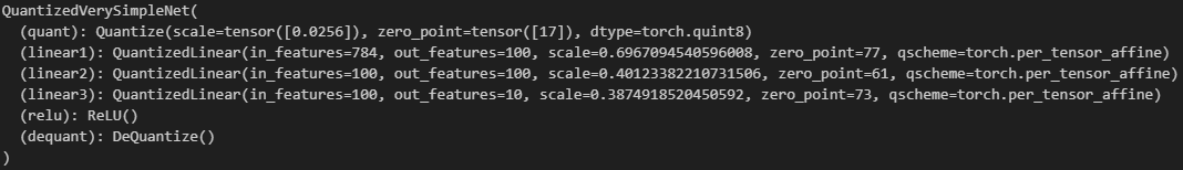
量化模型

# Quantize the model using the statistics collected

net_quantized = torch.ao.quantization.convert(net_quantized)

print(f'Check statistics of the various layers')
net_quantized

# Print the weights matrix of the model after quantization
print('Weights after quantization')
print(torch.int_repr(net_quantized.linear1.weight()))


# Compare the dequantized weights and the original weights
print('Original weights: ')
print(net.linear1.weight)
print('')
print(f'Dequantized weights: ')
print(torch.dequantize(net_quantized.linear1.weight()))
print('')

# Print size and accuracy of the quantized model
print('Size of the model after quantization')
print_size_of_model(net_quantized)
print('Testing the model after quantization')
test(net_quantized)