gtsam学习笔记2d SLAM(二)

最新推荐文章于 2023-12-29 09:19:25 发布

hex_refugeeeee

最新推荐文章于 2023-12-29 09:19:25 发布

阅读量787

点赞数

分类专栏：优化库 slam 文章标签：学习

本文链接：https://blog.csdn.net/weixin_45572737/article/details/128903330

版权

slam 同时被 2 个专栏收录

28 篇文章 15 订阅

订阅专栏

优化库

8 篇文章 1 订阅

订阅专栏

前言：

根据README.md里面的说明，对于2D Pose SLAM部分的example学习记录。

一、LocalizationExample.cpp

比较简单的一个例子：

在二维平面上有一个移动机器人，有它移动3个点时记录下来的gps数据，和这三个点之间的odometry的数据。然后给定一个错误的初值，最后求得结果和前面设置的gps数据对比。

unaryFactor设置

// Before we begin the example, we must create a custom unary factor to implement a

// "GPS-like" functionality. Because standard GPS measurements provide information

// only on the position, and not on the orientation, we cannot use a simple prior to

// properly model this measurement.

就是说用标准的gps是只有position坐标，没有orientation信息，所以就需要创建一个unaryFactor类。

具体代码如下：

class UnaryFactor: public NoiseModelFactor1<Pose2> {

  // The factor will hold a measurement consisting of an (X,Y) location
  // We could this with a Point2 but here we just use two doubles
  double mx_, my_;

public:
  /// shorthand for a smart pointer to a factor
  typedef boost::shared_ptr<UnaryFactor> shared_ptr;

  // The constructor requires the variable key, the (X, Y) measurement value, and the noise model
  UnaryFactor(Key j, double x, double y, const SharedNoiseModel& model):
    NoiseModelFactor1<Pose2>(model, j), mx_(x), my_(y) {}

  virtual ~UnaryFactor() {}

  // Using the NoiseModelFactor1 base class there are two functions that must be overridden.
  // The first is the 'evaluateError' function. This function implements the desired measurement
  // function, returning a vector of errors when evaluated at the provided variable value. It
  // must also calculate the Jacobians for this measurement function, if requested.
  Vector evaluateError(const Pose2& q, boost::optional<Matrix&> H = boost::none) const
  {
    // The measurement function for a GPS-like measurement is simple:
    // error_x = pose.x - measurement.x
    // error_y = pose.y - measurement.y
    // Consequently, the Jacobians are:
    // [ derror_x/dx  derror_x/dy  derror_x/dtheta ] = [1 0 0]
    // [ derror_y/dx  derror_y/dy  derror_y/dtheta ] = [0 1 0]
    if (H) (*H) = (Matrix(2,3) << 1.0,0.0,0.0, 0.0,1.0,0.0).finished();
    return (Vector(2) << q.x() - mx_, q.y() - my_).finished();
  }

  // The second is a 'clone' function that allows the factor to be copied. Under most
  // circumstances, the following code that employs the default copy constructor should
  // work fine.
  virtual gtsam::NonlinearFactor::shared_ptr clone() const {
    return boost::static_pointer_cast<gtsam::NonlinearFactor>(
        gtsam::NonlinearFactor::shared_ptr(new UnaryFactor(*this))); }

  // Additionally, we encourage you the use of unit testing your custom factors,
  // (as all GTSAM factors are), in which you would need an equals and print, to satisfy the
  // GTSAM_CONCEPT_TESTABLE_INST(T) defined in Testable.h, but these are not needed below.

}; // UnaryFactor

比较简单，值得注意的是如果要继承NoiseModelFactor1，需要override两个函数evaluateError和clone。

具体执行过程：

int main(int argc, char** argv) {

  // 1. Create a factor graph container and add factors to it
  NonlinearFactorGraph graph;

  // 2a. Add odometry factors
  // For simplicity, we will use the same noise model for each odometry factor
  noiseModel::Diagonal::shared_ptr odometryNoise = noiseModel::Diagonal::Sigmas(Vector3(0.2, 0.2, 0.1));
  // Create odometry (Between) factors between consecutive poses
  graph.emplace_shared<BetweenFactor<Pose2> >(1, 2, Pose2(2.0, 0.0, 0.0), odometryNoise);
  graph.emplace_shared<BetweenFactor<Pose2> >(2, 3, Pose2(3.0, 0.0, 0.0), odometryNoise);

  // 2b. Add "GPS-like" measurements
  // We will use our custom UnaryFactor for this.
  noiseModel::Diagonal::shared_ptr unaryNoise = noiseModel::Diagonal::Sigmas(Vector2(0.1, 0.1)); // 10cm std on x,y
  graph.emplace_shared<UnaryFactor>(1, 0.0, 0.0, unaryNoise);
  graph.emplace_shared<UnaryFactor>(2, 2.0, 0.0, unaryNoise);
  graph.emplace_shared<UnaryFactor>(3, 5.0, 0.0, unaryNoise);
  graph.print("\nFactor Graph:\n"); // print

  // 3. Create the data structure to hold the initialEstimate estimate to the solution
  // For illustrative purposes, these have been deliberately set to incorrect values
  Values initialEstimate;
  initialEstimate.insert(1, Pose2(0.5, 0.0, 0.2));
  initialEstimate.insert(2, Pose2(2.3, 0.1, -0.2));
  initialEstimate.insert(3, Pose2(4.1, 0.1, 0.1));
  initialEstimate.print("\nInitial Estimate:\n"); // print

  // 4. Optimize using Levenberg-Marquardt optimization. The optimizer
  // accepts an optional set of configuration parameters, controlling
  // things like convergence criteria, the type of linear system solver
  // to use, and the amount of information displayed during optimization.
  // Here we will use the default set of parameters.  See the
  // documentation for the full set of parameters.
  LevenbergMarquardtOptimizer optimizer(graph, initialEstimate);
  Values result = optimizer.optimize();
  result.print("Final Result:\n");

  // 5. Calculate and print marginal covariances for all variables
  Marginals marginals(graph, result);
  cout << "x1 covariance:\n" << marginals.marginalCovariance(1) << endl;
  cout << "x2 covariance:\n" << marginals.marginalCovariance(2) << endl;
  cout << "x3 covariance:\n" << marginals.marginalCovariance(3) << endl;

  return 0;
}

第一步创建graph；

第二步往graph里面添加odometry factor，添加GPS-like的factor；

第三步设置Values，初值initialEstimate，添加一些数；

第四步选择优化器，优化并输出结果。

结果：

Factor Graph:
size: 5

Factor 0: BetweenFactor(1,2)
  measured: (2, 0, 0)
  noise model: diagonal sigmas[0.2; 0.2; 0.1];

Factor 1: BetweenFactor(2,3)
  measured: (3, 0, 0)
  noise model: diagonal sigmas[0.2; 0.2; 0.1];

Factor 2:   keys = { 1 }
isotropic dim=2 sigma=0.1

Factor 3:   keys = { 2 }
isotropic dim=2 sigma=0.1

Factor 4:   keys = { 3 }
isotropic dim=2 sigma=0.1


Initial Estimate:
Values with 3 values:
Value 1: (N5gtsam5Pose2E) (0.5, 0, 0.2)

Value 2: (N5gtsam5Pose2E) (2.3, 0.1, -0.2)

Value 3: (N5gtsam5Pose2E) (4.1, 0.1, 0.1)

Final Result:
Values with 3 values:
Value 1: (N5gtsam5Pose2E) (-1.34728301e-14, 1.16725243e-15, -1.64808921e-16)

Value 2: (N5gtsam5Pose2E) (2, 2.17285499e-16, -7.22571183e-17)

Value 3: (N5gtsam5Pose2E) (5, -2.19538393e-16, -7.00766967e-17)

x1 covariance:
  0.00828571429  2.76564799e-19 -7.47383061e-19
 2.76564799e-19   0.00928571429  -0.00261904762
-7.47383061e-19  -0.00261904762   0.00706349206
x2 covariance:
 0.00714285714 1.61131272e-19 1.17630708e-19
1.61131272e-19  0.00801587302 -0.00134920635
1.17630708e-19 -0.00134920635  0.00468253968
x3 covariance:
 0.00828571429 1.35379321e-19 2.35144668e-19
1.35379321e-19  0.00968253968  0.00253968254
2.35144668e-19  0.00253968254   0.0146825397

可以看出，虽然在添加odometry和gps factor中添加了nosiy，但最后输出的结果是符合真实值的。

二、Pose2SLAMExample.cpp

这个内容很简单，有一个2d平面，然后机器人在里面运行，记录了5个点之间的里程计信息。通过优化，求解它们相对于第一个点的坐标信息。

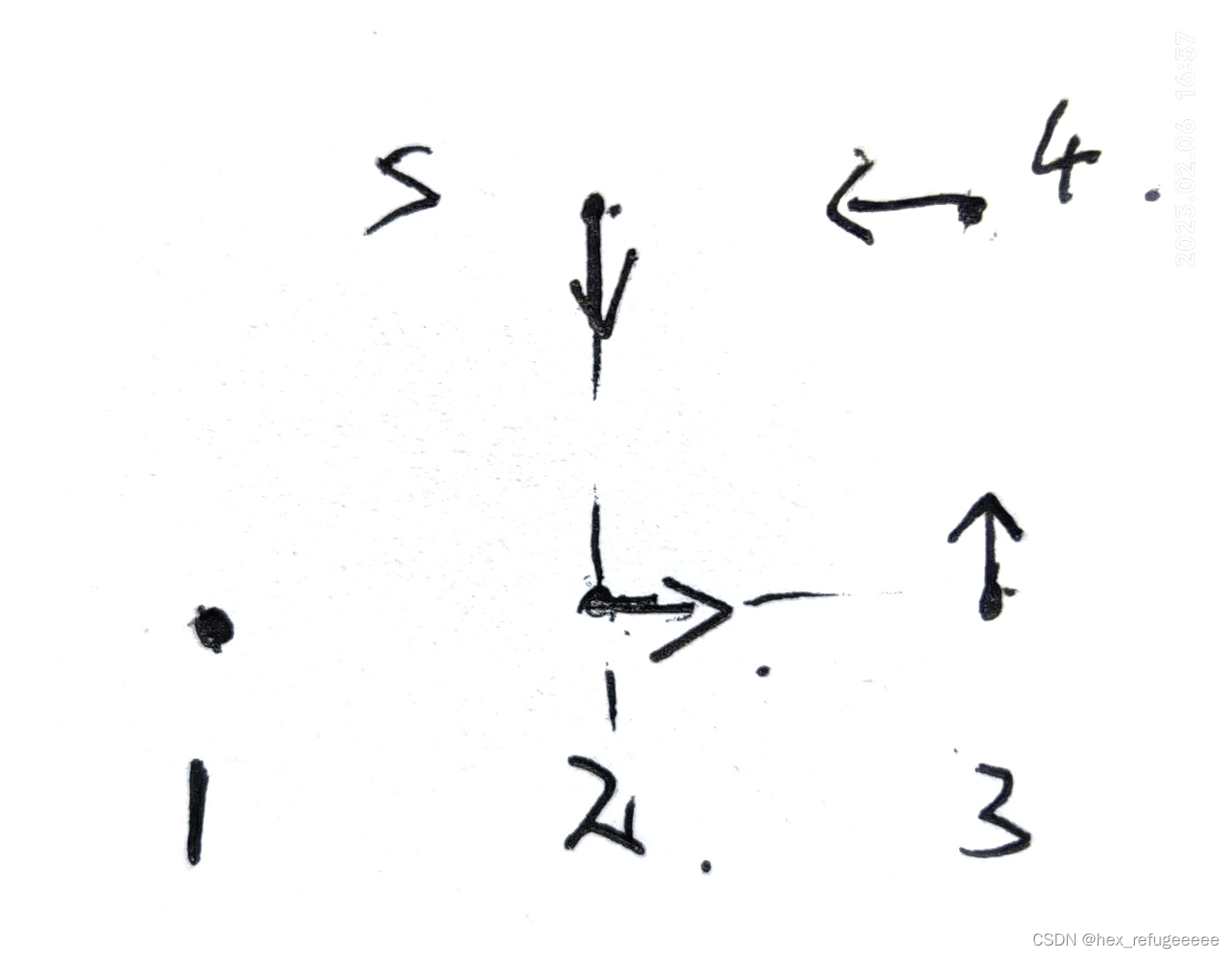
就是这个图的意思。

第一步：创建graph

  // 1. Create a factor graph container and add factors to it
  NonlinearFactorGraph graph;

第二步：创建factor

  // 2a. Add a prior on the first pose, setting it to the origin
  // A prior factor consists of a mean and a noise model (covariance matrix)
  noiseModel::Diagonal::shared_ptr priorNoise = noiseModel::Diagonal::Sigmas(Vector3(0.3, 0.3, 0.1));
  graph.emplace_shared<PriorFactor<Pose2> >(1, Pose2(0, 0, 0), priorNoise);

  // For simplicity, we will use the same noise model for odometry and loop closures
  noiseModel::Diagonal::shared_ptr model = noiseModel::Diagonal::Sigmas(Vector3(0.2, 0.2, 0.1));

  // 2b. Add odometry factors
  // Create odometry (Between) factors between consecutive poses
  graph.emplace_shared<BetweenFactor<Pose2> >(1, 2, Pose2(2, 0, 0     ), model);
  graph.emplace_shared<BetweenFactor<Pose2> >(2, 3, Pose2(2, 0, M_PI_2), model);
  graph.emplace_shared<BetweenFactor<Pose2> >(3, 4, Pose2(2, 0, M_PI_2), model);
  graph.emplace_shared<BetweenFactor<Pose2> >(4, 5, Pose2(2, 0, M_PI_2), model);

  // 2c. Add the loop closure constraint
  // This factor encodes the fact that we have returned to the same pose. In real systems,
  // these constraints may be identified in many ways, such as appearance-based techniques
  // with camera images. We will use another Between Factor to enforce this constraint:
  graph.emplace_shared<BetweenFactor<Pose2> >(5, 2, Pose2(2, 0, M_PI_2), model);
  graph.print("\nFactor Graph:\n"); // print

包括创建第一个因子和回环限制因子。

第三步：创建初值，并确定输出的数据类型和初值的格式一样。

  // 3. Create the data structure to hold the initialEstimate estimate to the solution
  // For illustrative purposes, these have been deliberately set to incorrect values
  Values initialEstimate;
  initialEstimate.insert(1, Pose2(0.5, 0.0,  0.2   ));
  initialEstimate.insert(2, Pose2(2.3, 0.1, -0.2   ));
  initialEstimate.insert(3, Pose2(4.1, 0.1,  M_PI_2));
  initialEstimate.insert(4, Pose2(4.0, 2.0,  M_PI  ));
  initialEstimate.insert(5, Pose2(2.1, 2.1, -M_PI_2));
  initialEstimate.print("\nInitial Estimate:\n"); // print

第四步：优化

  // 4. Optimize the initial values using a Gauss-Newton nonlinear optimizer
  // The optimizer accepts an optional set of configuration parameters,
  // controlling things like convergence criteria, the type of linear
  // system solver to use, and the amount of information displayed during
  // optimization. We will set a few parameters as a demonstration.
  GaussNewtonParams parameters;
  // Stop iterating once the change in error between steps is less than this value
  parameters.relativeErrorTol = 1e-5;
  // Do not perform more than N iteration steps
  parameters.maxIterations = 100;
  // Create the optimizer ...
  GaussNewtonOptimizer optimizer(graph, initialEstimate, parameters);
  // ... and optimize
  Values result = optimizer.optimize();
  result.print("Final Result:\n");

与之前不同的是，多了对于优化器参数的设置部分。

第五步：查看方差

  // 5. Calculate and print marginal covariances for all variables
  cout.precision(3);
  Marginals marginals(graph, result);
  cout << "x1 covariance:\n" << marginals.marginalCovariance(1) << endl;
  cout << "x2 covariance:\n" << marginals.marginalCovariance(2) << endl;
  cout << "x3 covariance:\n" << marginals.marginalCovariance(3) << endl;
  cout << "x4 covariance:\n" << marginals.marginalCovariance(4) << endl;
  cout << "x5 covariance:\n" << marginals.marginalCovariance(5) << endl;

简单明了，最容易理解的就是这个。

结果：

Final Result:
Values with 5 values:
Value 1: (N5gtsam5Pose2E) (-1.27455483e-20, 8.10527674e-20, 3.07189987e-20)

Value 2: (N5gtsam5Pose2E) (2, 1.78514217e-19, 4.34262714e-20)

Value 3: (N5gtsam5Pose2E) (4, -3.42173202e-11, 1.57079633)

Value 4: (N5gtsam5Pose2E) (4, 2, 3.14159265)

Value 5: (N5gtsam5Pose2E) (2, 2, -1.57079633)

三、Pose2SLAMExampleExpressions.cpp

这个和二的Pose2SLAMExample.cpp区别不大，主要的区别是使用：

  // Create Expressions for unknowns
  Pose2_ x1(1), x2(2), x3(3), x4(4), x5(5);

来代替了Pose2SLAMExample.cpp里面的数字1，2，3，4，5。

以及ExpressionFactorGraph来替代了NonlinearFactorGraph。

  ExpressionFactorGraph graph;

结果都一样：

Final Result:
Values with 5 values:
Value 1: (N5gtsam5Pose2E) (1.49017327e-20, -2.14141805e-20, -4.58273596e-21)

Value 2: (N5gtsam5Pose2E) (2, -4.0097066e-20, -4.40676513e-21)

Value 3: (N5gtsam5Pose2E) (4, -4.9189295e-12, 1.57079633)

Value 4: (N5gtsam5Pose2E) (4, 2, -3.14159265)

Value 5: (N5gtsam5Pose2E) (2, 2, -1.57079633)

四、Pose2SLAMExample_g2o.cpp

读取g2o文件的内容然后直接输出计算，和前面的类似。

example中的源码部分使用了很多封装的函数比如readG2o，输入g2o文件名和3d标志位，输出已经将factor加入的graph和已经添加了的初值initial指针。

    boost::tie(graph, initial) = readG2o(g2oFile,is3D);

/**
 * @brief This function parses a g2o file and stores the measurements into a
 * NonlinearFactorGraph and the initial guess in a Values structure
 * @param filename The name of the g2o file\
 * @param is3D indicates if the file describes a 2D or 3D problem
 * @param kernelFunctionType whether to wrap the noise model in a robust kernel
 * @return graph and initial values
 */
GTSAM_EXPORT GraphAndValues readG2o(const std::string& g2oFile, const bool is3D = false,
    KernelFunctionType kernelFunctionType = KernelFunctionTypeNONE);

还有writeG2o函数：

/**
 * @brief This function writes a g2o file from
 * NonlinearFactorGraph and a Values structure
 * @param filename The name of the g2o file to write
 * @param graph NonlinearFactor graph storing the measurements
 * @param estimate Values
 */
GTSAM_EXPORT void writeG2o(const NonlinearFactorGraph& graph,
    const Values& estimate, const std::string& filename);

其他部分和前面的一样，这里只是多了对于txt文件的读取和封装函数readG2o的使用。

完整源码：

#include <gtsam/slam/dataset.h>
#include <gtsam/slam/PriorFactor.h>
#include <gtsam/geometry/Pose2.h>
#include <gtsam/nonlinear/GaussNewtonOptimizer.h>
#include <fstream>

using namespace std;
using namespace gtsam;

// HOWTO: ./Pose2SLAMExample_g2o inputFile outputFile (maxIterations) (tukey/huber)
int main(const int argc, const char *argv[]) {

  string kernelType = "none";
  int maxIterations = 100; // default
  string g2oFile = findExampleDataFile("noisyToyGraph.txt"); // default

  // Parse user's inputs
  if (argc > 1){
    g2oFile = argv[1]; // input dataset filename
    // outputFile = g2oFile = argv[2]; // done later
  }
  if (argc > 3){
    maxIterations = atoi(argv[3]); // user can specify either tukey or huber
  }
  if (argc > 4){
    kernelType = argv[4]; // user can specify either tukey or huber
  }

  // reading file and creating factor graph
  NonlinearFactorGraph::shared_ptr graph;
  Values::shared_ptr initial;
  bool is3D = false;
  if(kernelType.compare("none") == 0){
    boost::tie(graph, initial) = readG2o(g2oFile,is3D);
  }
  if(kernelType.compare("huber") == 0){
    std::cout << "Using robust kernel: huber " << std::endl;
    boost::tie(graph, initial) = readG2o(g2oFile,is3D, KernelFunctionTypeHUBER);
  }
  if(kernelType.compare("tukey") == 0){
    std::cout << "Using robust kernel: tukey " << std::endl;
    boost::tie(graph, initial) = readG2o(g2oFile,is3D, KernelFunctionTypeTUKEY);
  }


  // Add prior on the pose having index (key) = 0
  NonlinearFactorGraph graphWithPrior = *graph;
  noiseModel::Diagonal::shared_ptr priorModel = //
      noiseModel::Diagonal::Variances(Vector3(1e-6, 1e-6, 1e-8));
  graphWithPrior.add(PriorFactor<Pose2>(0, Pose2(), priorModel));
  std::cout << "Adding prior on pose 0 " << std::endl;
  graphWithPrior.print("\nFactor Graph:\n");

  GaussNewtonParams params;
  params.setVerbosity("TERMINATION");
  if (argc > 3) {
    params.maxIterations = maxIterations;
    std::cout << "User required to perform maximum  " << params.maxIterations << " iterations "<< std::endl;
  }

  std::cout << "initial data: " << std::endl;
  (*initial).print("\nInitial Estimate:\n");

  std::cout << "Optimizing the factor graph" << std::endl;
  GaussNewtonOptimizer optimizer(graphWithPrior, *initial, params);
  Values result = optimizer.optimize();
  std::cout << "Optimization complete" << std::endl;

  // std::cout << "initial error=" <<graph->error(*initial)<< std::endl;
  // std::cout << "final error=" <<graph->error(result)<< std::endl;

  if (argc < 3) {
    result.print("result");
  } else {
    const string outputFile = argv[2];
    std::cout << "Writing results to file: " << outputFile << std::endl;
    NonlinearFactorGraph::shared_ptr graphNoKernel;
    Values::shared_ptr initial2;
    boost::tie(graphNoKernel, initial2) = readG2o(g2oFile);
    writeG2o(*graphNoKernel, result, outputFile);
    std::cout << "done! " << std::endl;
  }
  return 0;
}

原始部分没有对于加入graph的输出和初值initial的输出提示，我加了进去。

输出结果：

Factor Graph:
size: 6

Factor 0: BetweenFactor(0,1)
  measured: (0.774115, 1.18339, 1.57617)
  noise model: unit (3) 

Factor 1: BetweenFactor(1,2)
  measured: (0.869231, 1.03188, 1.57942)
  noise model: unit (3) 

Factor 2: BetweenFactor(2,3)
  measured: (1.35784, 1.03426, 1.56646)
  noise model: unit (3) 

Factor 3: BetweenFactor(2,0)
  measured: (0.303492, 1.86501, -3.1139)
  noise model: unit (3) 

Factor 4: BetweenFactor(0,3)
  measured: (-0.928526, 0.993695, -1.56354)
  noise model: unit (3) 

Factor 5: PriorFactor on 0
  prior mean: (0, 0, 0)
  noise model: diagonal sigmas[0.001; 0.001; 0.0001];

initial data: 

Initial Estimate:
Values with 4 values:
Value 0: (N5gtsam5Pose2E) (0, 0, 0)

Value 1: (N5gtsam5Pose2E) (0.774115, 1.183389, 1.576173)

Value 2: (N5gtsam5Pose2E) (-0.26242, 2.047059, -3.127594)

Value 3: (N5gtsam5Pose2E) (-1.605649, 0.993891, -1.561134)

Optimizing the factor graph
Warning:  stopping nonlinear iterations because error increased
errorThreshold: 0.0685034665 <? 0
absoluteDecrease: -2.28853697639e-05 <? 1e-05
relativeDecrease: -0.000334187727181 <? 1e-05
iterations: 3 >? 100
Optimization complete
resultValues with 4 values:
Value 0: (N5gtsam5Pose2E) (-7.53875248522e-23, -3.04401700725e-24, 1.41745664019e-24)

Value 1: (N5gtsam5Pose2E) (0.956178940406, 1.14319822891, 1.54150026689)

Value 2: (N5gtsam5Pose2E) (0.126611466178, 1.9817945338, -3.08397402066)

Value 3: (N5gtsam5Pose2E) (-1.05038303244, 0.935131621066, -1.54052801033)

然后，我根据Pose2SLAMExampleExpressions.cpp的内容，使用这个noisyToyGraph.txt文件的内容，写了个类似的，手动输入值。

#include <gtsam/slam/expressions.h>
#include <gtsam/nonlinear/ExpressionFactorGraph.h>
#include <gtsam/slam/PriorFactor.h>
#include <gtsam/slam/BetweenFactor.h>
#include <gtsam/geometry/Pose2.h>
#include <gtsam/nonlinear/GaussNewtonOptimizer.h>
#include <gtsam/nonlinear/Marginals.h>

using namespace std;
using namespace gtsam;

int main(int argc, char** argv)
{
    ExpressionFactorGraph graph;
    Pose2_ x1(1), x2(2), x3(3), x4(4);

    noiseModel::Diagonal::shared_ptr priorNoise = noiseModel::Diagonal::Sigmas(Vector3(0.3, 0.3, 0.1));
    graph.addExpressionFactor(x1, Pose2(0, 0, 0), priorNoise);

    noiseModel::Diagonal::shared_ptr model = noiseModel::Diagonal::Sigmas(Vector3(0.2, 0.2, 0.1));      

    graph.addExpressionFactor(between(x1,x2), Pose2(0.774115, 1.183389, 1.576173), model);
    graph.addExpressionFactor(between(x2,x3), Pose2(0.869231, 1.031877, 1.579418), model);
    graph.addExpressionFactor(between(x3,x4), Pose2(1.357840, 1.034262, 1.566460), model);
    graph.addExpressionFactor(between(x3,x1), Pose2(0.303492, 1.865011, -3.113898), model);
    graph.addExpressionFactor(between(x1,x4), Pose2(-0.928526, 0.993695, -1.563542), model);

    graph.print("\nFactor Graph:\n"); // print

    Values initialEstimate;   
    initialEstimate.insert(1, Pose2(0.0, 0.0,  0.0   ));
    initialEstimate.insert(2, Pose2(0.774115, 1.183389, 1.576173   ));
    initialEstimate.insert(3, Pose2(-0.262420, 2.047059, -3.127594));
    initialEstimate.insert(4, Pose2(-1.605649, 0.993891,  -1.561134  ));
    initialEstimate.print("\nInitial Estimate:\n"); // print

    GaussNewtonParams parameters;
    parameters.relativeErrorTol = 1e-5;
    parameters.maxIterations = 3;
    GaussNewtonOptimizer optimizer(graph, initialEstimate, parameters);
    Values result = optimizer.optimize();
    result.print("Final Result:\n");

    return 0;
}

发现它们的结果不一样，不知道是哪里出现了问题。

//我自己写的
Values with 4 values:
Value 1: (N5gtsam5Pose2E) (-2.22725181e-16, 4.72511144e-17, 2.13599316e-17)

Value 2: (N5gtsam5Pose2E) (0.986584345, 1.13382604, 1.56093936)

Value 3: (N5gtsam5Pose2E) (0.175794601, 1.96362262, -3.12403007)

Value 4: (N5gtsam5Pose2E) (-1.04609988, 0.949686099, -1.56055604)

//使用Pose2SLAMExample_g2o.cpp输出的
resultValues with 4 values:
Value 0: (N5gtsam5Pose2E) (-7.53875248522e-23, -3.04401700725e-24, 1.41745664019e-24)

Value 1: (N5gtsam5Pose2E) (0.956178940406, 1.14319822891, 1.54150026689)

Value 2: (N5gtsam5Pose2E) (0.126611466178, 1.9817945338, -3.08397402066)

Value 3: (N5gtsam5Pose2E) (-1.05038303244, 0.935131621066, -1.54052801033)

五、Pose2SLAMExample_graph.cpp

主要是读取w100.graph文件内容的example，和前面没有太多的不同，有一个封装函数load2D，

  boost::tie(graph, initial) = load2D(graph_file, model);

输入graph_file文件和nosiy model，输出是已经将factor加入的graph和已经加入的初值initial。其它类似前面的。

六、Pose2SLAMExample_graphviz.cpp

这部分的主要内容和Pose2SLAMExample.cpp一模一样，它不同在于介绍了一个函数：

  // save factor graph as graphviz dot file
  // Render to PDF using "fdp Pose2SLAMExample.dot -Tpdf > graph.pdf"
  ofstream os("Pose2SLAMExample.dot");
  graph.saveGraph(os, result);

可以将获得的结果result存放在os文件中，并通过命令：

fdp Pose2SLAMExample.dot -Tpdf > graph.pdf

将它转换为PDF文件。

对比initial值：

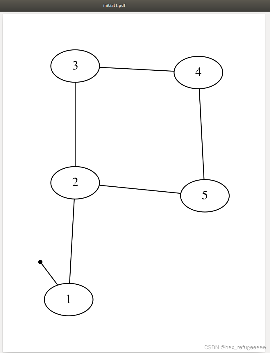
优化的效果还是很明显的。

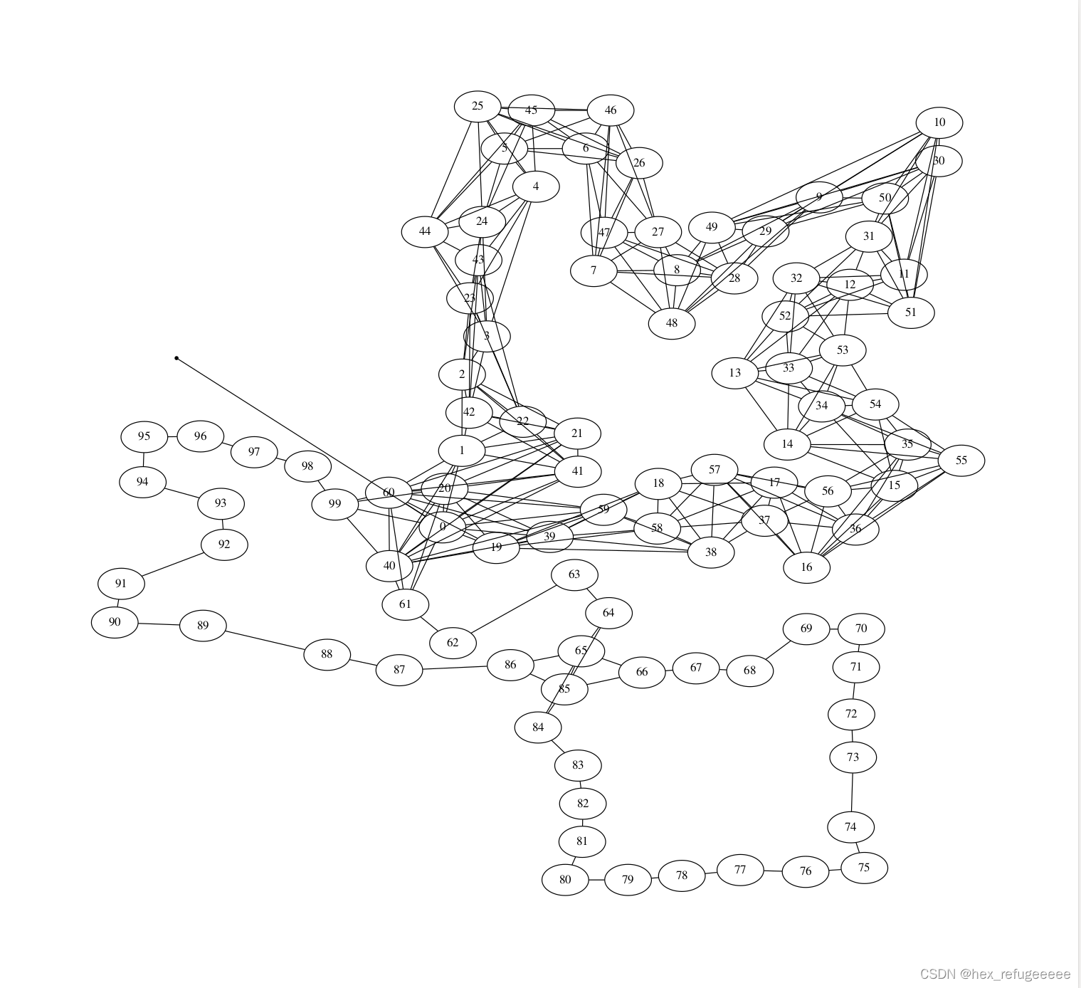
我利用这个函数和命令把前面w100.graph的优化结果也显示了一下：

七、Pose2SLAMStressTest.cpp

这个好像是创造一系列的3D poses，每个pose都加入噪声，然后就优化？

// Create N 3D poses, add relative motion between each consecutive poses. (The

// relative motion is simply a unit translation(1, 0, 0), no rotation). For each

// each pose, add some random noise to the x value of the translation part.

// Use gtsam to create a prior factor for the first pose and N-1 between factors

// and run optimization.

比较简单，对于initial部分的添加偏差值得学习一下：

  std::random_device rd;
  std::mt19937 e2(rd());
  std::uniform_real_distribution<> dist(0, 1);

  vector<Pose3> poses;
  for (int i = 0; i < numberNodes; ++i) {
    Matrix4 M;
    double r = dist(e2);
    r = (r - 0.5) / 10 + i;
    M << 1, 0, 0, r, 0, 1, 0, 0, 0, 0, 1, 0, 0, 0, 0, 1;
    poses.push_back(Pose3(M));
  }

八、Pose2SLAMwSPCG.cpp

使用了PCG solver来求解，其他内容和Pose2SLAMExample.cpp部分一样。

  // 4. Single Step Optimization using Levenberg-Marquardt
  LevenbergMarquardtParams parameters;
  parameters.verbosity = NonlinearOptimizerParams::ERROR;
  parameters.verbosityLM = LevenbergMarquardtParams::LAMBDA;

  // LM is still the outer optimization loop, but by specifying "Iterative" below
  // We indicate that an iterative linear solver should be used.
  // In addition, the *type* of the iterativeParams decides on the type of
  // iterative solver, in this case the SPCG (subgraph PCG)
  parameters.linearSolverType = NonlinearOptimizerParams::Iterative;
  parameters.iterativeParams = boost::make_shared<SubgraphSolverParameters>();

就是使用了sub PCG的求解，具体为什么使用这个不太清楚。