


WGCNA 简明指南|1. 基因共表达网络构建及模块识别
参考
简介
数据导入、清洗及预处理
数据导入
检查过度缺失值和离群样本
载入临床特征数据
自动构建网络及识别模块
确定合适的软阈值:网络拓扑分析
一步构建网络和识别模块
往期
参考
本文主要参考官方指南Tutorials for WGCNA R package (ucla.edu),详细内容可参阅官方文档。
其它资料:
WGCNA - 文集 - 简书 (jianshu.com)
WGCNA分析,简单全面的最新教程 - 简书 (jianshu.com)
简介
加权基因共表达网络分析 (WGCNA, Weighted correlation network analysis)是用来描述不同样品之间基因关联模式的系统生物学方法,可以用来鉴定高度协同变化的基因集, 并根据基因集的内连性和基因集与表型之间的关联鉴定候补生物标记基因或治疗靶点。简而言之,就是将基因划分为若干个模块,探究表型数据与基因模块之间的相关关系,并找到模块中的hub基因。
数据导入、清洗及预处理
数据导入
示例数据下载:https://horvath.genetics.ucla.edu/html/CoexpressionNetwork/Rpackages/WGCNA/Tutorials/FemaleLiver-Data.zip
# BiocManager::install("WGCNA")
library('WGCNA')
# 在读入数据时,遇到字符串之后,不将其转换为factors,仍然保留为字符串格式
options(stringsAsFactors = FALSE)
# 导入示例数据
femData = read.csv("LiverFemale3600.csv")
# 查看数据
dim(femData)
names(femData)
> dim(femData)
[1] 3600 143
> names(femData)
[1] "substanceBXH" "gene_symbol" "LocusLinkID" "ProteomeID"
[5] "cytogeneticLoc" "CHROMOSOME" "StartPosition" "EndPosition"
[9] "F2_2" "F2_3" "F2_14" "F2_15"
...# 提取样本-基因表达矩阵
datExpr0 = as.data.frame(t(femData[, -c(1:8)]))
names(datExpr0) = femData$substanceBXH
rownames(datExpr0) = names(femData)[-c(1:8)]> datExpr0[1:6,1:6]
MMT00000044 MMT00000046 MMT00000051 MMT00000076 MMT00000080 MMT00000102
F2_2 -0.0181000 -0.0773 -0.02260000 -0.00924 -0.04870000 0.17600000
F2_3 0.0642000 -0.0297 0.06170000 -0.14500 0.05820000 -0.18900000
F2_14 0.0000644 0.1120 -0.12900000 0.02870 -0.04830000 -0.06500000
F2_15 -0.0580000 -0.0589 0.08710000 -0.04390 -0.03710000 -0.00846000
F2_19 0.0483000 0.0443 -0.11500000 0.00425 0.02510000 -0.00574000
F2_20 -0.1519741 -0.0938 -0.06502607 -0.23610 0.08504274 -0.01807182检查过度缺失值和离群样本
# 检查缺失值太多的基因和样本
gsg = goodSamplesGenes(datExpr0, verbose = 3);
gsg$allOK如果最后一个语句返回TRUE,则所有的基因都通过了检查。如果没有,我们就从数据中剔除不符合要求的基因和样本。
if(!gsg$allOK)
{
  #(可选)打印被删除的基因和样本名称:
  if(sum(!gsg$goodGenes)>0)
    printFlush(paste("Removinggenes:",paste(names(datExpr0)[!gsg$goodGenes], collapse =",")));
  if(sum(!gsg$goodSamples)>0)
    printFlush(paste("Removingsamples:",paste(rownames(datExpr0)[!gsg$goodSamples], collapse =",")));
  #删除不满足要求的基因和样本:
  datExpr0 = datExpr0[gsg$goodSamples, gsg$goodGenes]
}接下来,我们对样本进行聚类(与稍后的聚类基因相反),看看是否有任何明显的异常值。
sampleTree = hclust(dist(datExpr0), method ="average");
# 绘制样本树:打开一个尺寸为12 * 9英寸的图形输出窗口
# 可对窗口大小进行调整
sizeGrWindow(12,9)
# 如要保存可运行下面语句
# pdf(file="Plots/sampleClustering.pdf",width=12,height=9);
par(cex = 0.6)
par(mar =c(0,4,2,0))
plot(sampleTree, main ="Sampleclusteringtodetectoutliers",sub="", xlab="", cex.lab = 1.5,
cex.axis= 1.5, cex.main = 2)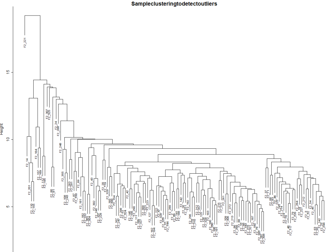
Fig1a可见有一个异常值。可以手动或使用自动方法删除它。选择一个**高度(height)**进行切割将删除异常样本,比如15(Fig1b),并在该高度使用分支切割
# 绘制阈值切割线
abline(h = 15,col="red");
# 确定阈值线下的集群
clust = cutreeStatic(sampleTree, cutHeight = 15, minSize = 10)
table(clust)
# clust1包含想要留下的样本.
keepSamples = (clust==1)
datExpr = datExpr0[keepSamples, ]
nGenes =ncol(datExpr)
nSamples =nrow(datExpr)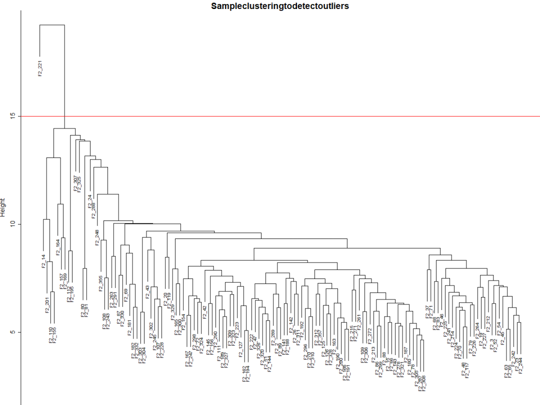
datExpr包含用于网络分析的表达数据。
载入临床特征数据
将样本信息与临床特征进行匹配。
traitData =read.csv("ClinicalTraits.csv")
dim(traitData)
names(traitData)
# 删除不必要的列.
allTraits = traitData[, -c(31, 16)]
allTraits = allTraits[,c(2, 11:36) ]
dim(allTraits)
names(allTraits)
# 形成一个包含临床特征的数据框
femaleSamples =rownames(datExpr)
traitRows =match(femaleSamples, allTraits$Mice)
datTraits = allTraits[traitRows, -1]
rownames(datTraits) = allTraits[traitRows, 1]
collectGarbage() # 释放内存现在在variabledatExpr中有了表达数据,在变量datTraits中有了相应的临床特征。在进行网络构建和模块检测之前,将临床特征与样本树状图的关系可视化。
# 重新聚类样本
sampleTree2 = hclust(dist(datExpr), method ="average")
# 将临床特征值转换为连续颜色:白色表示低,红色表示高,灰色表示缺失
traitColors = numbers2colors(datTraits, signed = FALSE);
# 在样本聚类图的基础上,增加临床特征值热图
plotDendroAndColors(sampleTree2, traitColors,
                    groupLabels =names(datTraits),
                    main ="Sample dendrogramand trait heatmap")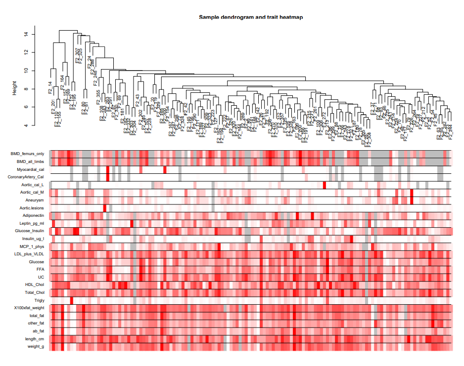
自动构建网络及识别模块
确定合适的软阈值:网络拓扑分析
The soft thresholding, is a value used to power the correlation of the genes to that threshold. The assumption on that by raising the correlation to a power will reduce the noise of the correlations in the adjacency matrix. To pick up one threshold use the pickSoftThreshold function, which calculates for each power if the network resembles to a scale-free graph. The power which produce a higher similarity with a scale-free network is the one you should use.
WGCNA: What is
soft thresholding? (bioconductor.org)
# 设置软阈值调参范围
powers =c(c(1:10),seq(from = 12, to=20,by=2))
# 网络拓扑分析
sft = pickSoftThreshold(datExpr, powerVector = powers, verbose = 5)
# 绘图
sizeGrWindow(9, 5)
# 1行2列排列
par(mfrow =c(1,2));
cex1 = 0.9;
# 无标度拓扑拟合指数与软阈值的函数(左图)
plot(sft$fitIndices[,1], -sign(sft$fitIndices[,3])*sft$fitIndices[,2],
     xlab="SoftThreshold(power)",ylab="ScaleFreeTopologyModelFit,signedR^2",type="n",
     main =paste("Scaleindependence"));
text(sft$fitIndices[,1], -sign(sft$fitIndices[,3])*sft$fitIndices[,2],
     labels=powers,cex=cex1,col="red");
# 这条线对应于h的R^2截止点
abline(h=0.90,col="red")
# Mean Connectivity与软阈值的函数(右图)
plot(sft$fitIndices[,1], sft$fitIndices[,5],
     xlab="SoftThreshold(power)",ylab="MeanConnectivity", type="n",
     main =paste("Meanconnectivity"))
text(sft$fitIndices[,1], sft$fitIndices[,5],labels=powers, cex=cex1,col="red")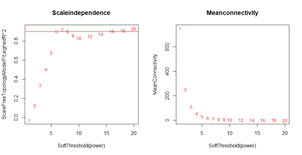
我们选择power 6,这是无标度拓扑拟合指数曲线在达到较高值时趋于平缓的最低 power。
一步构建网络和识别模块
net = blockwiseModules(datExpr,power= 6,
                       TOMType ="unsigned", minModuleSize = 30,
                       reassignThreshold = 0, mergeCutHeight = 0.25,
                       numericLabels = TRUE, pamRespectsDendro = FALSE,
                       saveTOMs = TRUE,
                       saveTOMFileBase ="femaleMouseTOM",
verbose = 3)deepSplit参数调整划分模块的敏感度,值越大,越敏感,得到的模块就越多,默认是2;minModuleSize参数设置最小模块的基因数,值越小,小的模块就会被保留下来;mergeCutHeight设置合并相似性模块的距离,值越小,就越不容易被合并,保留下来的模块就越多
# 查看识别了多少模块以及模块大小
table(net$colors)
> table(net$colors)
0 1 2 3 4 5 6 7 8 9 10 11 12 13 14 15 16 17 18
99 609 460 409 316 312 221 211 157 123 106 100 94 91 77 76 58 47 34表明有18个模块,按大小递减顺序标记为1到18,大小从609到34个基因。标签0为所有模块之外的基因。
# 可视化模块
sizeGrWindow(12, 9)
# 将标签转换为颜色
mergedColors = labels2colors(net$colors)
# 绘制树状图和模块颜色图
plotDendroAndColors(net$dendrograms[[1]], mergedColors[net$blockGenes[[1]]],
                    "Modulecolors",
                    dendroLabels = FALSE, hang = 0.03,
                    addGuide = TRUE, guideHang = 0.05)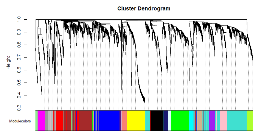
保存模块赋值和模块特征基因信息,以供后续分析。
moduleLabels = net$colors
moduleColors = labels2colors(net$colors)
MEs = net$MEs;
geneTree = net$dendrograms[[1]];
save(MEs, moduleLabels, moduleColors, geneTree,
     file="FemaleLiver-02-networkConstruction-auto.RData")
往期


 2138
2138

 被折叠的 条评论
为什么被折叠?
被折叠的 条评论
为什么被折叠?
 到【灌水乐园】发言


