R 实战 | 使用clusterProfiler进行多组基因富集分析

R 实战 | 使用clusterProfiler进行多组基因富集分析

clusterProfiler这个包我就不再介绍了，网上关于用这个包做的基础的富集分析的教程已经非常多了，今天主要介绍一下使用compareCluster功能进行多组基因的富集分析。

• 示例数据

• 富集分析

  • 多个基因集的富集分析

  • 多个分组的富集分析

• 基本用法

  • 参数

• References

• 往期

示例数据

library(clusterProfiler)
data(gcSample) #载入
str(gcSample) #数据集格式
lapply(gcSample, head) #查看数据集

> str(gcSample)
List of 8
 $ X1: chr [1:216] "4597" "7111" "5266" "2175" ...
 $ X2: chr [1:805] "23450" "5160" "7126" "26118" ...
 $ X3: chr [1:392] "894" "7057" "22906" "3339" ...
 $ X4: chr [1:838] "5573" "7453" "5245" "23450" ...
 $ X5: chr [1:929] "5982" "7318" "6352" "2101" ...
 $ X6: chr [1:585] "5337" "9295" "4035" "811" ...
 $ X7: chr [1:582] "2621" "2665" "5690" "3608" ...
 $ X8: chr [1:237] "2665" "4735" "1327" "3192" ...
> lapply(gcSample, head)
$X1
[1] "4597"  "7111"  "5266"  "2175"  "755"   "23046"

$X2
[1] "23450" "5160"  "7126"  "26118" "8452"  "3675" 

$X3
[1] "894"   "7057"  "22906" "3339"  "10449" "6566" 

$X4
[1] "5573"  "7453"  "5245"  "23450" "6500"  "4926" 

$X5
[1] "5982" "7318" "6352" "2101" "8882" "7803"

$X6
[1] "5337"  "9295"  "4035"  "811"   "23365" "4629" 

$X7
[1] "2621" "2665" "5690" "3608" "3550" "533" 

$X8
[1] "2665" "4735" "1327" "3192" "5573" "9528"

富集分析

多个基因集的富集分析

xx <- compareCluster(gcSample, fun="enrichKEGG",
                     organism="hsa", pvalueCutoff=0.05)
table(xx@compareClusterResult$Cluster) #每个基因集富集个数
head(as.data.frame(xx)) #查看完整结果

> table(xx@compareClusterResult$Cluster)

X1 X2 X3 X4 X5 X6 X7 X8 
 0  3  3 18 10  1 15 19 
> head(as.data.frame(xx))
  Cluster       ID                            Description GeneRatio
1      X2 hsa04110                             Cell cycle    18/384
2      X2 hsa05169           Epstein-Barr virus infection    23/384
3      X2 hsa05340               Primary immunodeficiency     8/384
4      X3 hsa04512               ECM-receptor interaction     9/187
5      X3 hsa04060 Cytokine-cytokine receptor interaction    17/187
6      X3 hsa04151             PI3K-Akt signaling pathway    19/187
   BgRatio       pvalue    p.adjust      qvalue
1 126/8105 2.441211e-05 0.007470105 0.006989572
2 202/8105 7.911793e-05 0.012105043 0.011326356
3  38/8105 3.297441e-04 0.033633898 0.031470314
4  88/8105 1.815667e-04 0.045098637 0.042158192
5 295/8105 4.490651e-04 0.045098637 0.042158192
6 354/8105 5.048355e-04 0.045098637 0.042158192
                                                                                                     geneID
1                   991/1869/890/1871/701/990/10926/9088/8317/9700/9134/1029/2810/699/11200/23594/8555/4173
2 4067/3383/7128/1869/890/1871/578/864/637/9641/6891/355/9134/5971/916/956/6850/7187/3551/919/4734/958/6772
3                                                                       100/6891/3932/973/916/925/958/64421
4                                                              7057/3339/1299/3695/1101/3679/3910/3696/3693
5                      2919/4982/3977/6375/8200/608/8792/3568/2057/1438/8718/655/652/10220/50615/51561/7042
6             894/7057/6794/2247/1299/3695/2252/2066/1101/8817/1021/5105/3679/3082/2057/3910/3551/3696/3693
  Count
1    18
2    23
3     8
4     9
5    17
6    19

dotplot(xx) #气泡图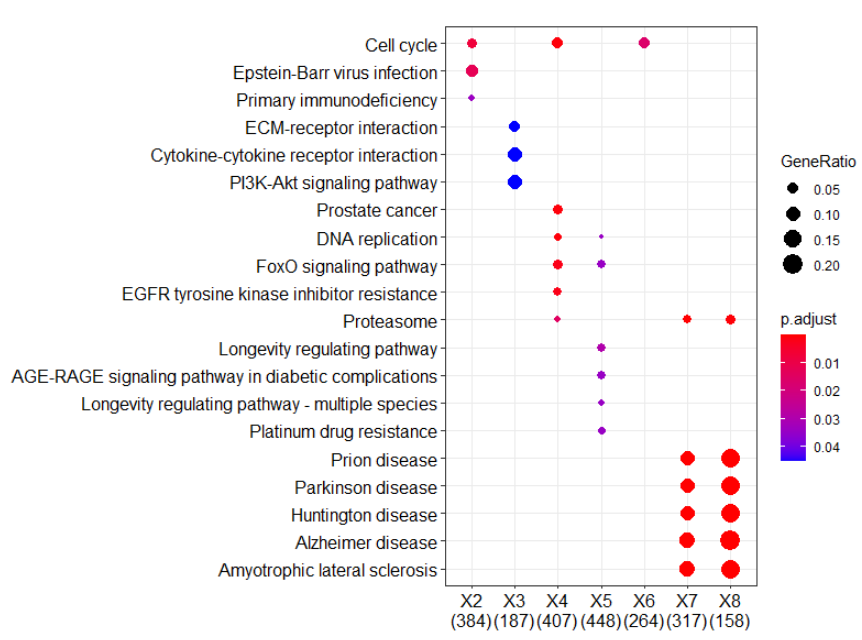

多个分组的富集分析

示例数据

data(geneList, package="DOSE") #载入DOSE包中的数据
head(geneList) #查看数据 包含基因名及其foldchange
mydf <- data.frame(Entrez=names(geneList), FC=geneList)
# 以下内容目的是构建分组 也可以用别的分组
# 将FC大于1的标注为上调 反之为下调
mydf <- mydf[abs(mydf$FC) > 1,]
mydf$group <- "upregulated"
mydf$group[mydf$FC < 0] <- "downregulated"
# 将FC绝对值大于2 的标注为B 反之为A
mydf$othergroup <- "A"
mydf$othergroup[abs(mydf$FC) > 2] <- "B"
head(mydf) # 查看示例数据(两个分组)

> head(mydf)
      Entrez       FC       group othergroup
4312    4312 4.572613 upregulated          B
8318    8318 4.514594 upregulated          B
10874  10874 4.418218 upregulated          B
55143  55143 4.144075 upregulated          B
55388  55388 3.876258 upregulated          B
991      991 3.677857 upregulated          B

分析及其可视化

# 可以进行单组或多组分析,在 + 号后添加即可
formula_res <- compareCluster(Entrez~group+othergroup, 
                              data=mydf, 
                              fun='enrichKEGG')
dotplot(formula_res)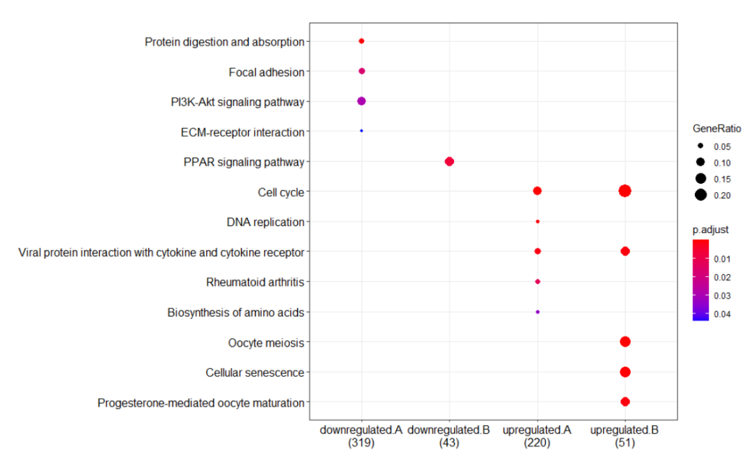

# 同样可以进行分面操作
dotplot(formula_res, x=~group) + 
  ggplot2::facet_grid(~othergroup) #对于只用一次该包的功能可以这么写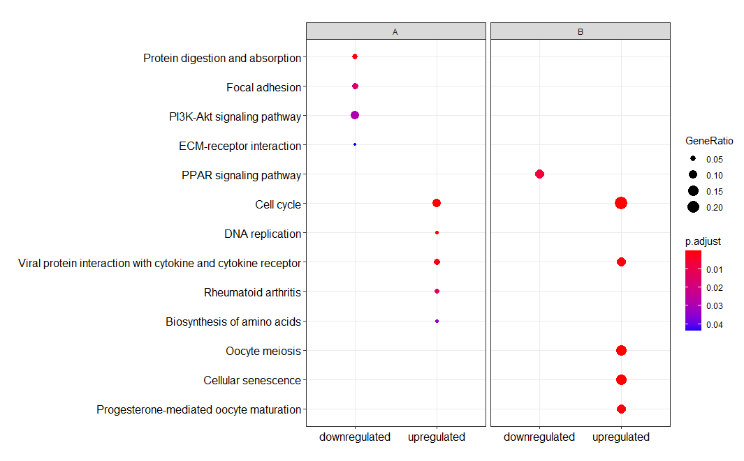

基本用法

最后附上用法参数。

compareCluster(geneClusters, fun = "enrichGO", data = "", ...)

参数

geneClusters	entrez基因list. 或者, Entrez~分组 形式的列表
fun	"groupGO", "enrichGO", "enrichKEGG", "enrichDO" or "enrichPathway" .
data	数据集

References

Chapter 11 Biological theme comparison | clusterProfiler: universal enrichment tool for functional and comparative study (hiplot.com.cn)

往期

R绘图实战|GSEA富集分析图

---