Seurat 4.0 | 单细胞转录组数据整合(scRNA-seq integration)

Seurat 4.0 | 单细胞转录组数据整合(scRNA-seq integration)

对于两个或多个单细胞数据集的整合问题，Seurat 自带一系列方法用于跨数据集匹配(match) (或“对齐” ,align)共享的细胞群。这些方法首先识别处于匹配生物状态的交叉数据集细胞(“锚”,anchors)，可以用于校正数据集之间的技术差异(如，批次效应校正)，也可以用于不同实验条件下的scRNA-seq的比较分析。

作者使用了两种不同状态(静息或干扰素刺激状态,a resting or interferon-stimulated state)的人类PBMC细胞进行比较分析作为示例。

整合目标

• 创建一个整合的assay用于下游分析

• 识别两个数据集中共有的细胞类型

• 获取在不同状态细胞中都保守的细胞标志物 (cell markers)

• 比较两个数据集,发现对刺激有反应(responses to stimulation)的细胞类型

设置Seurat对象

library(Seurat)
library(SeuratData) # 包含数据集
library(patchwork)

# 下载数据
InstallData("ifnb")

# 加载数据
LoadData("ifnb")
# 根据stim状态拆分为两个list (stim and CTRL)
ifnb.list <- SplitObject(ifnb, split.by = "stim")
ifnb.list

> ifnb.list
$CTRL
An object of class Seurat 
14053 features across 6548 samples within 1 assay 
Active assay: RNA (14053 features, 0 variable features)

$STIM
An object of class Seurat 
14053 features across 7451 samples within 1 assay 
Active assay: RNA (14053 features, 0 variable features)

可见，本方法的原始数据准备只需把不同condition或者tech的Seurat对象整合为一个list即可进行后续的分析。

# 分别对两个数据集进行标准化并识别变量特征
ifnb.list <- lapply(X = ifnb.list, FUN = function(x) {
    x <- NormalizeData(x)
    x <- FindVariableFeatures(x, selection.method = "vst", nfeatures = 2000)
})

# 选择跨数据集重复可变的特征进行整合
features <- SelectIntegrationFeatures(object.list = ifnb.list)

进行整合

FindIntegrationAnchors() 函数使用Seurat对象列表作为输入，来识别anchors。

IntegrateData() 函数使用识别到的anchors来整合数据集。

immune.anchors <- FindIntegrationAnchors(object.list = ifnb.list, anchor.features = features)

# 生成整合数据
immune.combined <- IntegrateData(anchorset = immune.anchors)

整合分析

#指定已校正的数据进行下游分析，注意未修改的原始数据仍在于 'RNA' assay中
DefaultAssay(immune.combined) <- "integrated"

# 标准数据可视化和分类流程
immune.combined <- ScaleData(immune.combined, verbose = FALSE)
immune.combined <- RunPCA(immune.combined, npcs = 30, verbose = FALSE)
immune.combined <- RunUMAP(immune.combined, reduction = "pca", dims = 1:30)
immune.combined <- FindNeighbors(immune.combined, reduction = "pca", dims = 1:30)
immune.combined <- FindClusters(immune.combined, resolution = 0.5)

# 可视化
p1 <- DimPlot(immune.combined, reduction = "umap", group.by = "stim")
p2 <- DimPlot(immune.combined, reduction = "umap", label = TRUE, repel = TRUE)
p1 + p2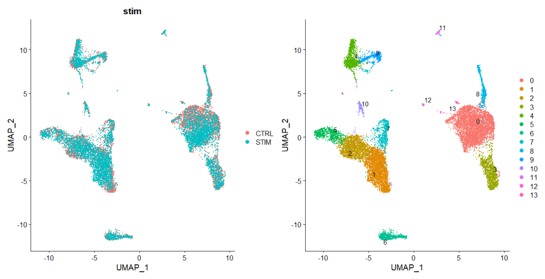

# split.by 展示分组聚类
DimPlot(immune.combined, reduction = "umap", split.by = "stim")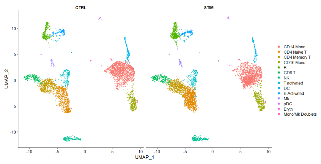

识别保守的细胞类型标记(markers)

使用 FindConservedMarkers() 函数识别在不同条件下保守的典型细胞类型标记基因. 例如，在cluster6 (NK细胞)中，我们可以计算出不受刺激条件影响的保守标记基因。

# 为了进行分组差异分析 将默认数据改为'RNA'
DefaultAssay(immune.combined) <- "RNA"
BiocManager::install('multtest')
install.packages('metap')
library(metap)
DefaultAssay(immune.combined) <- "RNA"
# ident.1设置聚类标签
nk.markers <- FindConservedMarkers(immune.combined, ident.1 = 6, grouping.var = "stim", verbose = FALSE)
head(nk.markers)

探索每个聚类的标记基因，使用标记基因注释细胞类型。

FeaturePlot(immune.combined, features = c("CD3D", "SELL", "CREM", "CD8A", "GNLY", "CD79A", "FCGR3A",
    "CCL2", "PPBP"), min.cutoff = "q9")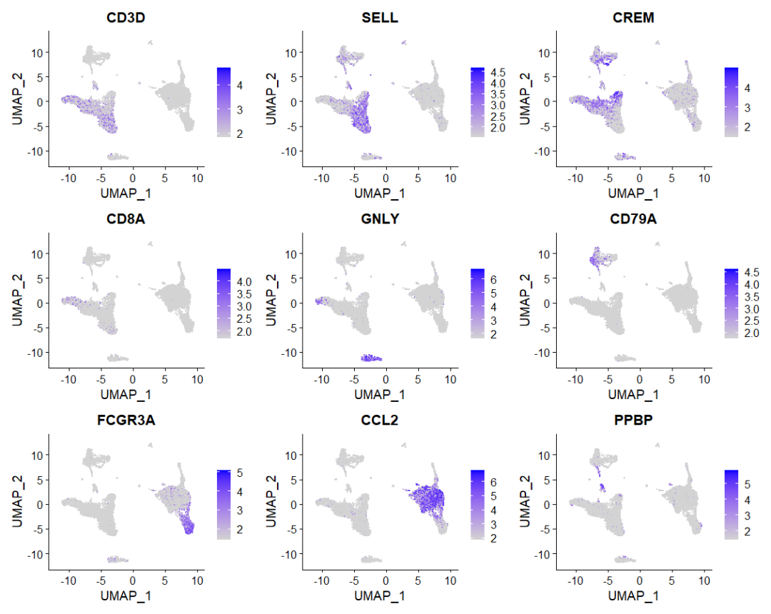

immune.combined <- RenameIdents(immune.combined, 
                                `0` = "CD14 Mono",
                                `1` = "CD4 Naive T", 
                                `2` = "CD4 Memory T",
                                `3` = "CD16 Mono", 
                                `4` = "B", 
                                `5` = "CD8 T", 
                                `6` = "NK",
                                `7` = "T activated",
                                `8` = "DC", 
                                `9` = "B Activated",
                                `10` = "Mk", 
                                `11` = "pDC", 
                                `12` = "Eryth", 
                                `13` = "Mono/Mk Doublets")
DimPlot(immune.combined, label = TRUE)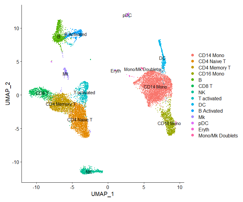

绘制标记基因气泡图

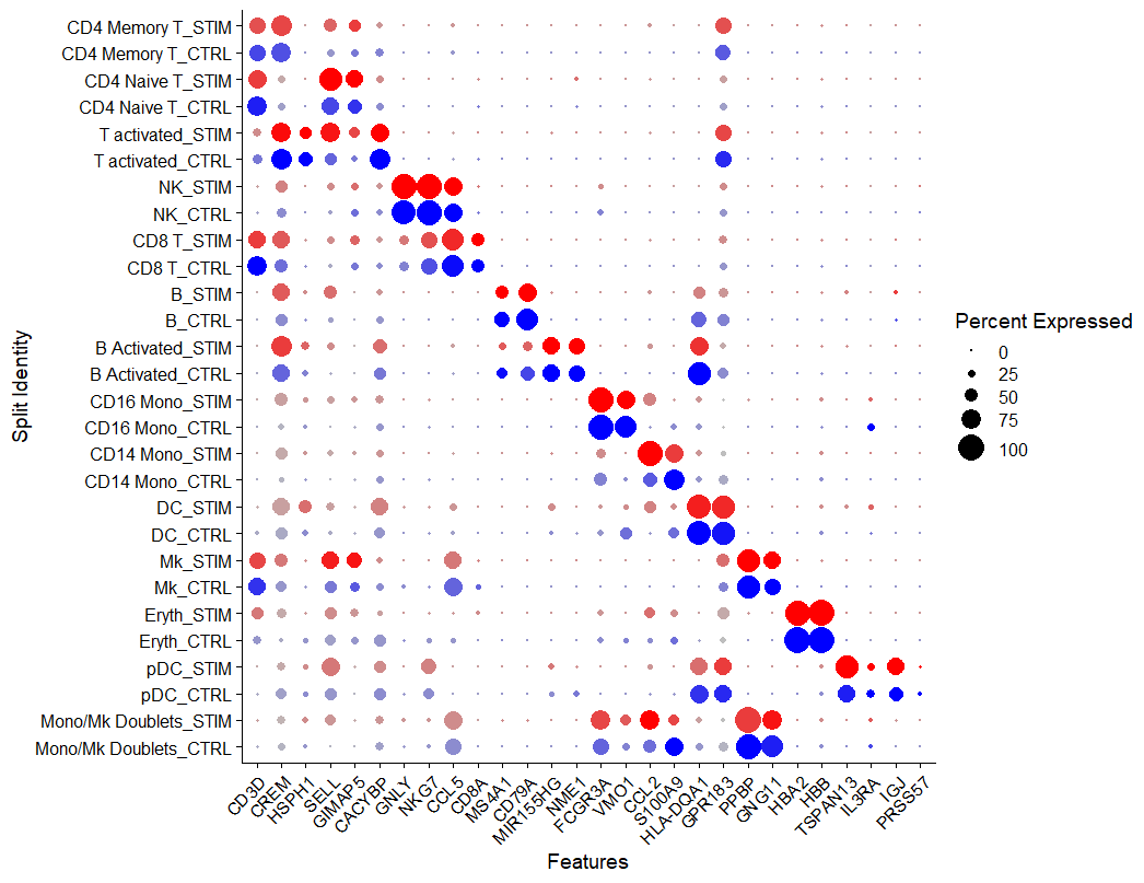
识别不同条件(condition)下的差异基因

library(ggplot2)
library(cowplot)
theme_set(theme_cowplot())

## CD4 Naive T
t.cells <- subset(immune.combined, idents = "CD4 Naive T")
Idents(t.cells) <- "stim"
avg.t.cells <- as.data.frame(log1p(AverageExpression(t.cells, verbose = FALSE)$RNA))
avg.t.cells$gene <- rownames(avg.t.cells)

## CD14 Mono
cd14.mono <- subset(immune.combined, idents = "CD14 Mono")
Idents(cd14.mono) <- "stim"
avg.cd14.mono <- as.data.frame(log1p(AverageExpression(cd14.mono, verbose = FALSE)$RNA))
avg.cd14.mono$gene <- rownames(avg.cd14.mono)

# 标签
genes.to.label = c("ISG15", "LY6E", "IFI6", "ISG20", "MX1", "IFIT2", "IFIT1", "CXCL10", "CCL8")

# 绘制
p1 <- ggplot(avg.t.cells, aes(CTRL, STIM)) + geom_point() + ggtitle("CD4 Naive T Cells")
p1 <- LabelPoints(plot = p1, points = genes.to.label, repel = TRUE)
p2 <- ggplot(avg.cd14.mono, aes(CTRL, STIM)) + geom_point() + ggtitle("CD14 Monocytes")
p2 <- LabelPoints(plot = p2, points = genes.to.label, repel = TRUE)
p1 + p2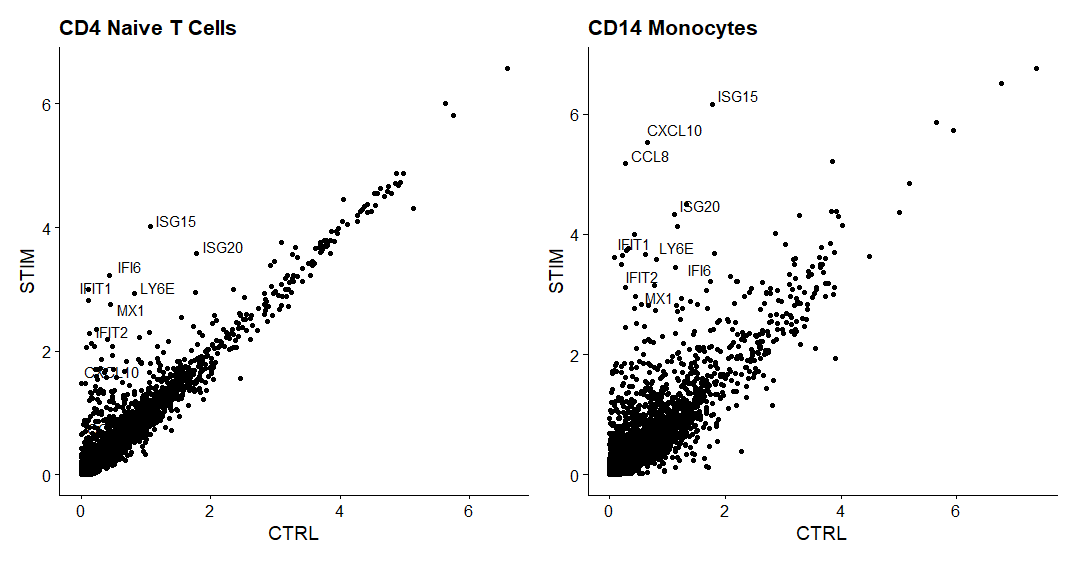

同一类型的细胞的不同条件下差异表达的基因。

immune.combined$celltype.stim <- paste(Idents(immune.combined), immune.combined$stim, sep = "_")
immune.combined$celltype <- Idents(immune.combined)
Idents(immune.combined) <- "celltype.stim"
table(immune.combined@active.ident)
## 对B细胞进行差异分析
b.interferon.response <- FindMarkers(immune.combined, ident.1 = "B_STIM", ident.2 = "B_CTRL", verbose = FALSE)
head(b.interferon.response, n = 15)

> head(b.interferon.response, n = 15)
                p_val avg_log2FC pct.1 pct.2     p_val_adj
ISG15   8.657899e-156  4.5965018 0.998 0.240 1.216695e-151
IFIT3   3.536522e-151  4.5004998 0.964 0.052 4.969874e-147
IFI6    1.204612e-149  4.2335821 0.966 0.080 1.692841e-145
ISG20   9.370954e-147  2.9393901 1.000 0.672 1.316900e-142
IFIT1   8.181640e-138  4.1290319 0.912 0.032 1.149766e-133
MX1     1.445540e-121  3.2932564 0.907 0.115 2.031417e-117
LY6E    2.944234e-117  3.1187120 0.894 0.152 4.137531e-113
TNFSF10 2.273307e-110  3.7772611 0.792 0.025 3.194678e-106
IFIT2   1.676837e-106  3.6547696 0.786 0.035 2.356459e-102
B2M      3.500771e-95  0.6062999 1.000 1.000  4.919633e-91
PLSCR1   3.279290e-94  2.8249220 0.797 0.117  4.608387e-90
IRF7     1.475385e-92  2.5888616 0.838 0.190  2.073358e-88
CXCL10   1.350777e-82  5.2509496 0.641 0.010  1.898247e-78
UBE2L6   2.783283e-81  2.1427434 0.851 0.300  3.911348e-77
PSMB9    2.638374e-76  1.6367800 0.941 0.573  3.707707e-72

## 可视化基因表达
FeaturePlot(immune.combined, features = c("CD3D", "GNLY", "IFI6"), split.by = "stim", max.cutoff = 3,
    cols = c("grey", "red"))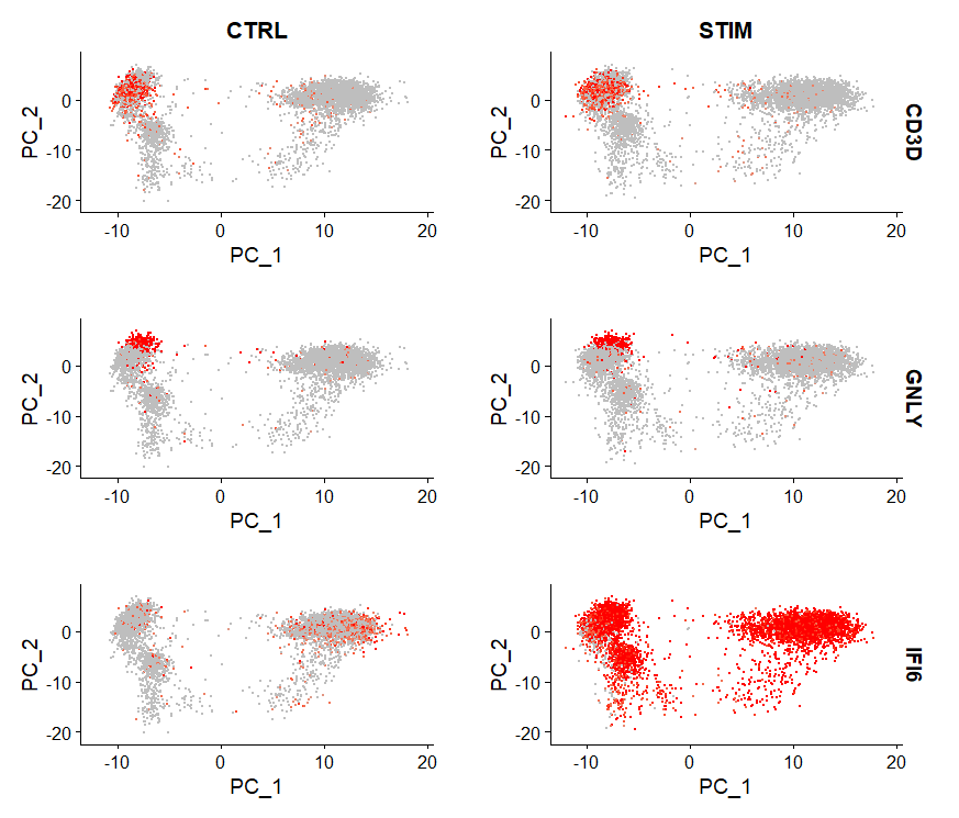

## 小提琴图
plots <- VlnPlot(immune.combined, features = c("LYZ", "ISG15", "CXCL10"), split.by = "stim", group.by = "celltype",
    pt.size = 0, combine = FALSE)
wrap_plots(plots = plots, ncol = 1)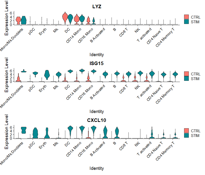

基于SCTransform标准化进行整合分析

SCTransform标准化流程主要差别在于：

• 使用SCTransform()标准化, 而不是 NormalizeData() 。

• 使用3,000 或更多的特征进入下游分析。

• 使用 PrepSCTIntegration()函数识别anchors。

• 当使用 FindIntegrationAnchors(), 和IntegrateData(), 将参数normalization.method 设置为 SCT。

• 运行基于sctransform的工作流程时，包括整合，不需要使用ScaleData()函数。

## 具体流程
LoadData("ifnb")
ifnb.list <- SplitObject(ifnb, split.by = "stim")
ifnb.list <- lapply(X = ifnb.list, FUN = SCTransform)
features <- SelectIntegrationFeatures(object.list = ifnb.list, nfeatures = 3000)
ifnb.list <- PrepSCTIntegration(object.list = ifnb.list, anchor.features = features)

immune.anchors <- FindIntegrationAnchors(object.list = ifnb.list, normalization.method = "SCT",
    anchor.features = features)
immune.combined.sct <- IntegrateData(anchorset = immune.anchors, normalization.method = "SCT")

immune.combined.sct <- RunPCA(immune.combined.sct, verbose = FALSE)
immune.combined.sct <- RunUMAP(immune.combined.sct, reduction = "pca", dims = 1:30)

p1 <- DimPlot(immune.combined.sct, reduction = "umap", group.by = "stim")
p2 <- DimPlot(immune.combined.sct, reduction = "umap", group.by = "seurat_annotations", label = TRUE,
    repel = TRUE)
p1 + p2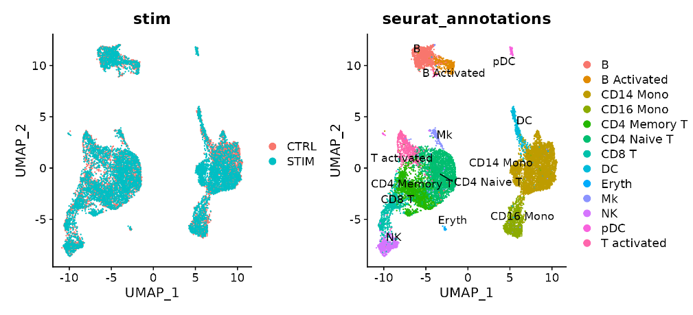

到此数据就整合结束了，后续可以接着前面的步骤进行细胞识别等分析。

参考

• https://satijalab.org/seurat/articles/integration_introduction.html

往期

• 单细胞转录组|Seurat 4.0 使用指南

- END -