【齿轮系统故障跟踪】基于现场测量的传递路径分析方法研究（Matlab代码实现）

👨‍🎓个人主页：研学社的博客  

💥💥💞💞欢迎来到本博客❤️❤️💥💥

🏆博主优势：🌞🌞🌞博客内容尽量做到思维缜密，逻辑清晰，为了方便读者。

⛳️座右铭：行百里者，半于九十。

📋📋📋本文目录如下：🎁🎁🎁

目录

💥1 概述

📚2 运行结果

2.1 通过虚拟解耦方法得到的FRF

2.2 识别轴承力及基于传递路径的信号分解

🎉3 参考文献

🌈4 Matlab代码实现

---

​

💥1 概述

本文主要研究齿轮系统的传递路径分析( TPA )。提出了一种虚拟解耦方法来实现基于原位测量的TPA。基于Tikhonov正则化理论进行了轴承力的识别。
采用一个齿轮动力学模型作为数值例子来说明传递路径分析的过程。关于所提出的TPA算法的细节可参见文献[1]。[1]。时变啮合刚度与动力学建模的互补信息见文献。[2、3]。

📚2 运行结果

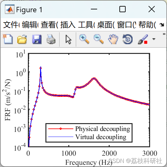
2.1 通过虚拟解耦方法得到的FRF

 

 

 

 

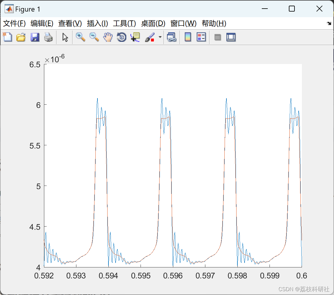
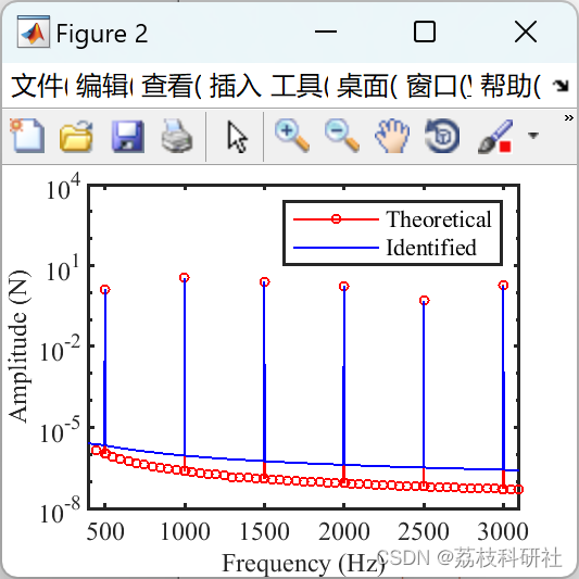
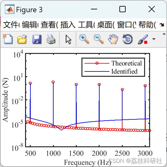
2.2 识别轴承力及基于传递路径的信号分解

 

 部分代码：

%% Project vector of the meshing element
V=[1,rb1,-1,rb2];
unit_VV=zeros(length(M));
unit_VV(1:4,1:4)=V'*V;
%% Stiffness and damping parameter of the spring-damping element
k15=1e7; k36=1e7; k57=1e8; k67=1e8; k07=1e8;
c15=1e4; c36=1e4; c57=1e3; c67=1e3; c07=1e3;
%% Matirx assembling of the whole system
K=zeros(length(M));
K([1,5],[1,5])=K([1,5],[1,5])+[k15,-k15;-k15,k15];
K([3,6],[3,6])=K([3,6],[3,6])+[k36,-k36;-k36,k36];
K([5,7],[5,7])=K([5,7],[5,7])+[k57,-k57;-k57,k57];
K([6,7],[6,7])=K([6,7],[6,7])+[k67,-k67;-k67,k67];
K(7,7)=K(7,7)+k07;

C=zeros(length(M));
C([1,5],[1,5])=C([1,5],[1,5])+[c15,-c15;-c15,c15];
C([3,6],[3,6])=C([3,6],[3,6])+[c36,-c36;-c36,c36];
C([5,7],[5,7])=C([5,7],[5,7])+[c57,-c57;-c57,c57];
C([6,7],[6,7])=C([6,7],[6,7])+[c67,-c67;-c67,c67];
C(7,7)=C(7,7)+c07;
%% Natural frequency of the whole system (coupled system)
K_mean=K+mean(K_health)*unit_VV;
D_whole=eig(K_mean/M);
Freq_whole=sqrt(sort(real(abs(D_whole))))/(2*pi);
%% Matirx assembling of the decoupled system (passive part)
Md=diag([m5,m6,m7]);

Kd=zeros(length(Md));
Kd([1,3],[1,3])=Kd([1,3],[1,3])+[k57,-k57;-k57,k57];
Kd([2,3],[2,3])=Kd([2,3],[2,3])+[k67,-k67;-k67,k67];
Kd(3,3)=Kd(3,3)+k07;

Cd=zeros(length(Md));
Cd([1,3],[1,3])=Cd([1,3],[1,3])+[c57,-c57;-c57,c57];
Cd([2,3],[2,3])=Cd([2,3],[2,3])+[c67,-c67;-c67,c67];
Cd(3,3)=Cd(3,3)+c07;
%% Natural frequency of the passive part (decoupled system)
Dd=eig(Kd/Md);
Freq_d=sqrt(sort(real(abs(Dd))))/(2*pi);
%% FRF analysis
Omega=linspace(1,12500*2*pi,4500);
DOF_a=[1,3];
DOF_p=[5,6];
for n=1:length(Omega)
    %% FRF of the passive part
    Hd=Omega(n)^2*inv(-Md*Omega(n)^2+Cd*1i*Omega(n)+Kd);   
    %% FRF of the whole system
    H=Omega(n)^2*inv(-M*Omega(n)^2+C*1i*Omega(n)+K_mean);   
    Hctp=H(7,DOF_p);
    Hcta=H(7,DOF_a);
    Hcaa=H(DOF_a,DOF_a);
    Hcpp=H(DOF_p,DOF_p);
    Hcpa=H(DOF_p,DOF_a);
    Hcap=H(DOF_a,DOF_p);   
    %% Virtual decoupling (estimated FRF)
    Hdtp=Hctp-Hcta*inv(Hcaa-Hcpa)*(Hcap-Hcpp); 
    %% Output
    Hdtp_real(:,n)=Hd([1,2],3);
    Hdpp_real(:,n)=Hd([1,2],1);
    Hdtp_estimated(:,n)=Hdtp;
end
%% Fig. 3 Comparison of FRF between the physical decoupling and virtual decoupling: (a) H57
figure(1)
% hold on
% plot(Omega(1:10:end)/2/pi,20*log10(abs(Hdtp_real(1,1:10:end))),'or','linewidth',0.75,'markersize',2)
% plot(Omega/2/pi,20*log10(abs(Hdtp_estimated(1,:))),'b','linewidth',0.75)

yy=semilogy(Omega(1:10:end)/2/pi,abs(Hdtp_real(1,1:10:end)),Omega/2/pi,abs(Hdtp_estimated(1,:)));
yy(1).Color=[1,0,0];
yy(1).Marker='o';
yy(1).LineWidth=0.75;
yy(1).MarkerSize=2;
yy(2).Color=[0,0,1];
yy(2).LineWidth=0.75;

set(gcf,'color','w','Units','centimeters','Position',[10 10 7 5]); 
set(gca,'fontname','Times New Roman','fontsize',9,'linewidth',1); 
box on
set(gca,'looseInset',[0 0 0.1 0]); % W S E N
xlabel('Frequency (Hz)','FontSize',9)
ylabel('FRF (m/s^2/N)','FontSize',9)
legend('Physical decoupling','Virtual decoupling','location','south')
xlim([0,3000])
ylim([10^-4,10^1])
set(gca,'YTick',[10^-4,10^-3,10^-2,10^-1,10^0,10^1])
%% Fig. 3 Comparison of FRF between the physical decoupling and virtual decoupling: (b) H67.
figure(2)
% hold on
% plot(Omega(1:10:end)/2/pi,20*log10(abs(Hdtp_real(2,1:10:end))),'or','linewidth',0.75,'markersize',2)
% plot(Omega/2/pi,20*log10(abs(Hdtp_estimated(2,:))),'b','linewidth',0.75)

yy=semilogy(Omega(1:10:end)/2/pi,abs(Hdtp_real(2,1:10:end)),Omega/2/pi,abs(Hdtp_estimated(2,:)));
yy(1).Color=[1,0,0];
yy(1).Marker='o';
yy(1).LineWidth=0.75;
yy(1).MarkerSize=2;
yy(2).Color=[0,0,1];
yy(2).LineWidth=0.75;

set(gcf,'color','w','Units','centimeters','Position',[10 10 7 5]); 
set(gca,'fontname','Times New Roman','fontsize',9,'linewidth',1); 
box on
set(gca,'looseInset',[0 0 0.1 0]); % W S E N
xlabel('Frequency (Hz)','FontSize',9)
ylabel('FRF (m/s^2/N)','FontSize',9)
legend('Physical decoupling','Virtual decoupling','location','south')
xlim([0,3000])
ylim([10^-4,10^1])
set(gca,'YTick',[10^-4,10^-3,10^-2,10^-1,10^0,10^1])
%%
% print -f1 -r600 -dpng figure1
% print -f2 -r600 -dpng figure2

% print -f1 '-dmeta' figure1
% print -f2 '-dmeta' figure2

🎉3 参考文献

部分理论来源于网络，如有侵权请联系删除。

1. Y.F. Huangfu, X.J. Dong, X.L. Yu, K.K. Chen, Z.W. Li, Z.K. Peng, Fault tracing of gear systems: An in-situ measurement-based transfer path analysis method, Journal of Sound and Vibration 553 (2023) 117610.1-26.
2. K.K. Chen, Y.F. Huangfu, H. Ma, Z.T. Xu, X. Li, B.C. Wen, Calculation of mesh stiffness of spur gears considering complex foundation types and crack propagation paths, Mechanical Systems and Signal Processing 130 (2019) 273-292.
3. Y.F. Huangfu, K.K. Chen, H. Ma, X. Li, H.Z. Han, Z.F. Zhao, Meshing and dynamic characteristics analysis of spalled gear systems: A theoretical and experimental study, Mechanical Systems and Signal Processing 139 (2020) 106640.1-21.

🌈4 Matlab代码实现