


💥💥💞💞欢迎来到本博客❤️❤️💥💥
🏆博主优势:🌞🌞🌞博客内容尽量做到思维缜密,逻辑清晰,为了方便读者。
⛳️座右铭:行百里者,半于九十。
📋📋📋本文目录如下:🎁🎁🎁
目录

💥1 概述
摘要:有限控制集模型预测控制(FCS-MPC)是功率转换系统的一种突出控制方法,最近非常受欢迎。一些研究强调了长预测范围在闭环稳定性、谐波失真和开关损耗方面实现的性能优势。然而,由于其固有的高计算负担,实际实现并不简单。为了克服这一障碍,可以将控制问题表述为整数最小二乘优化问题,相当于格中的最近点搜索或最近向量问题。文献中提出了不同的技术来解决它,其中球体解码算法(SDA)是解决长预测视界FCS-MPC的最流行选择。然而,该领域的最新技术提供了超越传统SDA的解决方案,本文将介绍这些解决方案以及该主题的未来趋势和挑战。
功率转换系统的控制是一个重要的研究领域,部分原因是可再生能源的增长以及将它们集成到电网中的需求[1],[2],[3]。电力电子和功率转换器的控制是实现向无碳发电过渡的关键方面。控制理论的进步转化为性能和效率的提高,这是进一步推动这些技术发展的关键[4]。
在这种范式中,模型预测控制(MPC)策略正在成为电力电子领域的一个突出研究课题[5],[6]。有几个因素可以解释这种比更传统的控制技术更受欢迎的原因。首先,MPC具有一个简单的公式,它提供了一种直观的方法来控制复杂系统。通过MPC技术,可以同时直观地考虑多个控制目标、系统非线性和约束。由于这些原因,研究工作提出了用于控制电力电子系统的不同MPC技术,包括广泛的功率转换器拓扑和应用[7],[8]。
在不同的MPC方法家族中,直接MPC或有限控制集MPC(FCS-MPC)因其与其他替代品相比更自然的配方而更受欢迎。在FCS-MPC中,功率转换器的分立特性被认为是一个整数优化问题,其中控制和调制在同一计算阶段中得到解决[9]。为此,控制输入仅限于电源转换器允许的开关状态。这组允许的输入就是所谓的有限控制集(FCS)。与连续控制集方法相比,一步法FCS-MPC的优化问题可以很容易地解决,例如,通过穷举枚举。这种方法也称为穷举搜索算法(ESA),是FCS-MPC应用中最常见的优化算法。ESA枚举FCS中每个可能的候选者,预测每个控制输入的未来状态,并评估成本函数以根据所选控制标准选择最佳开关位置[5]。由于计算成本,该策略在长预测视界(LPH)问题中暴露了其缺点。预测范围 (Np) 是预测中考虑的时间步长数。扩大Np开关状态的现有组合的数量呈指数级增长。因此,详尽的枚举变得难以处理。但是,更大的Np值意味着更长的预测窗口,该窗口为控制器提供附加信息。这一特征在更复杂的系统中尤其重要,
FCS-MPC依赖于后退的地平线政策[14];控制算法以离散时间步长以等于采样频率的速率执行fs.在每个时间步长,在上一个采样间隔中计算的最佳控制动作应用于功率转换器。这个过程在每个时间步重复,从系统中进行新的测量。此特性不会因扩展而改变Np.预测中考虑了更多的时间步长,但只有最佳序列中的第一个控制输入应用于功率转换器。
要定义FCS-MPC策略,需要三个基本要素:预测模型,成本函数和优化算法。预测模型计算系统状态变量在未来时间步长的演变,给定初始状态和可通过预测范围应用的可能控制输入序列。成本函数根据控制目标评估每个可能的轨迹和控制输入的适用性。优化算法最小化目标函数并选择控制输入的最佳顺序。
📚2 运行结果

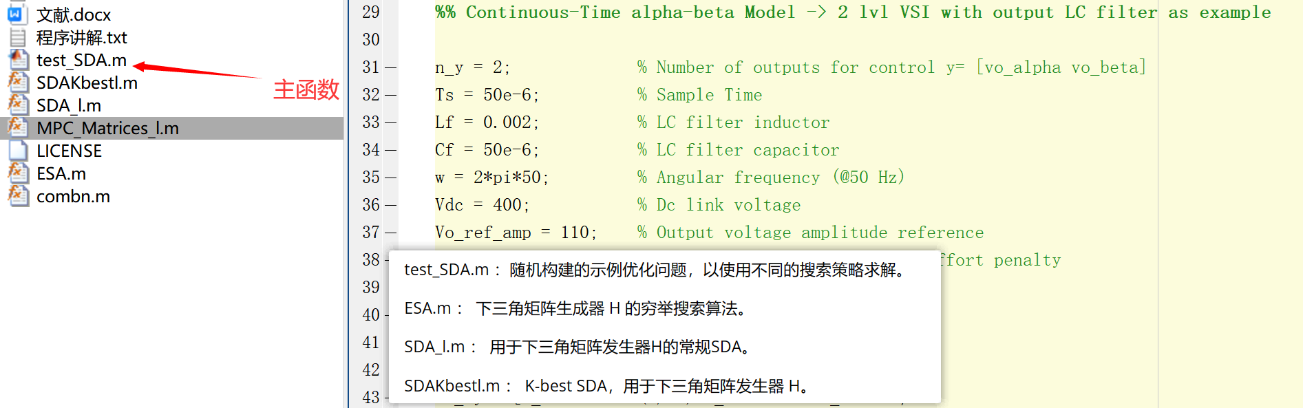
主函数代码:
clear all
clc
%% Original FCS
% \V = \{ u_{\min},...,u_{\max} \} \subset \Z
u_min=0;    %Minimum value for input
u_max=1;    %Maximum value for input

%% Multistep FCS
% u \in \V^n_u \subset \Z^n_u
% \U_k = \V^n_u Np \subset \Z^p; p=n_u Np

n_u = 3;             % Number of inputs u=[Sa Sb Sc]'
Np = 7;              % Prediction Horizon length
p = n_u*Np;          % Length of switching sequences U_k
Kbest = 8;           % Kb parameter for K-best SDA
Niter_max = 32000;   % Maximum number of explored nodes for SDA


%% Basic Matrices
I_2 = eye(2);          % Identity matrices
I_3 = eye(3);
O_2 = zeros(2);        % Zero matrices
J = [0 -1;
   1  0];
Tr = sqrt(2/3)*[1     -0.5         -0.5;      % Clarke transform
              0   sqrt(3)/2   -sqrt(3)/2];


%% Continuous-Time alpha-beta Model -> 2 lvl VSI with output LC filter as example

n_y = 2;             % Number of outputs for control y= [vo_alpha vo_beta]
Ts = 50e-6;          % Sample Time
Lf = 0.002;          % LC filter inductor
Cf = 50e-6;          % LC filter capacitor
w = 2*pi*50;         % Angular frequency (@50 Hz)
Vdc = 400;           % Dc link voltage
Vo_ref_amp = 110;    % Output voltage amplitude reference
lambda = 60.0;       % Weighting factor: Switching effort penalty

Rr=[1  -w*Ts;        % Rotation matrix
     w*Ts  1];

Ac_xy = [O_2        -(1/Lf)*I_2         O_2     ;
      (1/Cf)*I_2      O_2       -(1/Cf)*I_2   ;
       O_2            O_2             w*J     ;];

Bc_xy = [(Vdc/Lf)*I_2 O_2 O_2]'*Tr ;

Cxy = [I_2 O_2 O_2;
      O_2 I_2 O_2];   % C for observer

ct_sys = ss(Ac_xy,Bc_xy,Cxy,[]);

%% Discrete-Time alpha-beta Model
dt_sys = c2d(ct_sys,Ts);
A = dt_sys.a;
B = dt_sys.b;


%% Multistep Matrices (H is lower triangular)
C = zeros(n_y,6);        % C for control, 2 rows because only voltage is controlled
C(1:n_y,3:4) = eye(2);

[UpsilonT,Gamma,lSTE,W_inv,H] = MPC_Matrices_l(A,B,C,Np,lambda); %Multistep matrices


%% Initialize variables
Uop_ESA = zeros(p,1);
Uop_SDA = zeros(p,1);
Uop_Kbest = zeros(p,1);
F_k=zeros(p,1);
Niter=0.0;           % Count nodes
Niter_ac=0.0;
Niter_avg=0.0;
sim = 0;             % Number of simulations
simMAX = 1;
uabc_k_1 = [0 0 0]'; % Assume previous state is 0 0 0

while (sim < simMAX)

%% Vo Reference
theta = 2*pi*(rand(1));     % Syncronization angle, generated randomly in this example
Vo_abc_ref = Vo_ref_amp*[sin(theta); sin(theta-2*pi/3); sin(theta+2*pi/3)];
Vo_xy_ref = Tr*Vo_abc_ref;  % Vo reference in alpha-beta

%% Output sequences
Yref=zeros(n_y*Np,1);
Yref(1:2,1)=Rr*Vo_xy_ref;   % Construct output reference sequence

for k=n_y+1:n_y:n_y*Np
    row_i=k;
    row_f=k+n_y-1;

    Yref(row_i:row_f,:)=Rr*Yref(row_i-n_y:row_f-n_y,:);
end

%% System state
Vo_xy = Vo_xy_ref + 20*(rand(1)-0.5);       % Assume Vo around reference with +-10 V error
Io_xy = [0 0]';                             % Assume output current is zero
Ii_xy = Io_xy + (Cf/Ts)*(Rr*Vo_xy-Vo_xy);   % Approximate filter current

x_k = [Ii_xy ; Vo_xy; Io_xy];               % System state variables


%% Unconstrained solution calculation
F_k=UpsilonT*(Gamma*x_k-Yref)-lSTE*uabc_k_1;
U_unc=-W_inv*F_k;
%U_unc = 4*(rand(p,1)-0.5); % To generate randomly
%U_unc = min(u_max+1, max(u_min-1, U_unc)); % Limit unconstrained values
U_bar_unc = H*U_unc;          % Center of the sphere in the transformed space

%% Initial Vector U_ini -> Only for SDA
U_ini = zeros(p,1);               % Null vector
%U_vec_ini=round(U_vec_unc);    % Babai
% for k =1 : p
%    if (U_vec_ini(k,1)<u_min)
%        U_vec_ini(k,1)=u_min;
%    end
%    if (U_vec_ini(k,1)>u_max)
%        U_vec_ini(k,1)=u_max;
%    end
% end


%% Exhaustive Search Algorithm
Uop_ESA = ESA(U_bar_unc, H, u_min, u_max, p);

%% Sphere Decoding Algorithm
[Uop_SDA,Niter,Rs2] = SDA_l(U_bar_unc, H, u_min, u_max, p, U_ini,Niter_max);

%% K-best Sphere Decoding Algorithm
[Uop_Kbest,NiterKb,Rs2Kb] = SDAKbestl(U_bar_unc, H, u_min, u_max, p,Kbest);

Uop_ESA'
Uop_SDA'
Niter
Uop_Kbest'
NiterKb

Niter_ac=Niter_ac+Niter;
sim = sim+1;

end

Niter_avg=Niter_ac/sim;
clear all
clc
%% Original FCS
% \V = \{ u_{\min},...,u_{\max} \} \subset \Z
u_min=0; %Minimum value for input
u_max=1; %Maximum value for input
%% Multistep FCS
% u \in \V^n_u \subset \Z^n_u
% \U_k = \V^n_u Np \subset \Z^p; p=n_u Np
n_u = 3; % Number of inputs u=[Sa Sb Sc]'
Np = 7; % Prediction Horizon length
p = n_u*Np; % Length of switching sequences U_k
Kbest = 8; % Kb parameter for K-best SDA
Niter_max = 32000; % Maximum number of explored nodes for SDA
%% Basic Matrices
I_2 = eye(2); % Identity matrices
I_3 = eye(3);
O_2 = zeros(2); % Zero matrices
J = [0 -1;
1 0];
Tr = sqrt(2/3)*[1 -0.5 -0.5; % Clarke transform
0 sqrt(3)/2 -sqrt(3)/2];
%% Continuous-Time alpha-beta Model -> 2 lvl VSI with output LC filter as example
n_y = 2; % Number of outputs for control y= [vo_alpha vo_beta]
Ts = 50e-6; % Sample Time
Lf = 0.002; % LC filter inductor
Cf = 50e-6; % LC filter capacitor
w = 2*pi*50; % Angular frequency (@50 Hz)
Vdc = 400; % Dc link voltage
Vo_ref_amp = 110; % Output voltage amplitude reference
lambda = 60.0; % Weighting factor: Switching effort penalty
Rr=[1 -w*Ts; % Rotation matrix
w*Ts 1];
Ac_xy = [O_2 -(1/Lf)*I_2 O_2 ;
(1/Cf)*I_2 O_2 -(1/Cf)*I_2 ;
O_2 O_2 w*J ;];
Bc_xy = [(Vdc/Lf)*I_2 O_2 O_2]'*Tr ;
Cxy = [I_2 O_2 O_2;
O_2 I_2 O_2]; % C for observer
ct_sys = ss(Ac_xy,Bc_xy,Cxy,[]);
%% Discrete-Time alpha-beta Model
dt_sys = c2d(ct_sys,Ts);
A = dt_sys.a;
B = dt_sys.b;
%% Multistep Matrices (H is lower triangular)
C = zeros(n_y,6); % C for control, 2 rows because only voltage is controlled
C(1:n_y,3:4) = eye(2);
[UpsilonT,Gamma,lSTE,W_inv,H] = MPC_Matrices_l(A,B,C,Np,lambda); %Multistep matrices
%% Initialize variables
Uop_ESA = zeros(p,1);
Uop_SDA = zeros(p,1);
Uop_Kbest = zeros(p,1);
F_k=zeros(p,1);
Niter=0.0; % Count nodes
Niter_ac=0.0;
Niter_avg=0.0;
sim = 0; % Number of simulations
simMAX = 1;
uabc_k_1 = [0 0 0]'; % Assume previous state is 0 0 0
while (sim < simMAX)
%% Vo Reference
theta = 2*pi*(rand(1)); % Syncronization angle, generated randomly in this example
Vo_abc_ref = Vo_ref_amp*[sin(theta); sin(theta-2*pi/3); sin(theta+2*pi/3)];
Vo_xy_ref = Tr*Vo_abc_ref; % Vo reference in alpha-beta
%% Output sequences
Yref=zeros(n_y*Np,1);
Yref(1:2,1)=Rr*Vo_xy_ref; % Construct output reference sequence
for k=n_y+1:n_y:n_y*Np
row_i=k;
row_f=k+n_y-1;
Yref(row_i:row_f,:)=Rr*Yref(row_i-n_y:row_f-n_y,:);
end
%% System state
Vo_xy = Vo_xy_ref + 20*(rand(1)-0.5); % Assume Vo around reference with +-10 V error
Io_xy = [0 0]'; % Assume output current is zero
Ii_xy = Io_xy + (Cf/Ts)*(Rr*Vo_xy-Vo_xy); % Approximate filter current
x_k = [Ii_xy ; Vo_xy; Io_xy]; % System state variables
%% Unconstrained solution calculation
F_k=UpsilonT*(Gamma*x_k-Yref)-lSTE*uabc_k_1;
U_unc=-W_inv*F_k;
%U_unc = 4*(rand(p,1)-0.5); % To generate randomly
%U_unc = min(u_max+1, max(u_min-1, U_unc)); % Limit unconstrained values
U_bar_unc = H*U_unc; % Center of the sphere in the transformed space
%% Initial Vector U_ini -> Only for SDA
U_ini = zeros(p,1); % Null vector
%U_vec_ini=round(U_vec_unc); % Babai
% for k =1 : p
% if (U_vec_ini(k,1)<u_min)
% U_vec_ini(k,1)=u_min;
% end
% if (U_vec_ini(k,1)>u_max)
% U_vec_ini(k,1)=u_max;
% end
% end
%% Exhaustive Search Algorithm
Uop_ESA = ESA(U_bar_unc, H, u_min, u_max, p);
%% Sphere Decoding Algorithm
[Uop_SDA,Niter,Rs2] = SDA_l(U_bar_unc, H, u_min, u_max, p, U_ini,Niter_max);
%% K-best Sphere Decoding Algorithm
[Uop_Kbest,NiterKb,Rs2Kb] = SDAKbestl(U_bar_unc, H, u_min, u_max, p,Kbest);
Uop_ESA'
Uop_SDA'
Niter
Uop_Kbest'
NiterKb
Niter_ac=Niter_ac+Niter;
sim = sim+1;
end
Niter_avg=Niter_ac/sim;
🎉3 参考文献
文章中一些内容引自网络,会注明出处或引用为参考文献,难免有未尽之处,如有不妥,请随时联系删除。


 7153
7153


 被折叠的 条评论
为什么被折叠?
被折叠的 条评论
为什么被折叠?
 到【灌水乐园】发言


