【无人机】采用NOMA的节能多无人机多接入边缘计算（Matlab代码实现）

👨‍🎓个人主页：研学社的博客  

💥💥💞💞欢迎来到本博客❤️❤️💥💥

🏆博主优势：🌞🌞🌞博客内容尽量做到思维缜密，逻辑清晰，为了方便读者。

⛳️座右铭：行百里者，半于九十。

📋📋📋本文目录如下：🎁🎁🎁

目录

💥1 概述

📚2 运行结果

🎉3 参考文献

🌈4 Matlab代码实现

---

💥1 概述

文献来源：

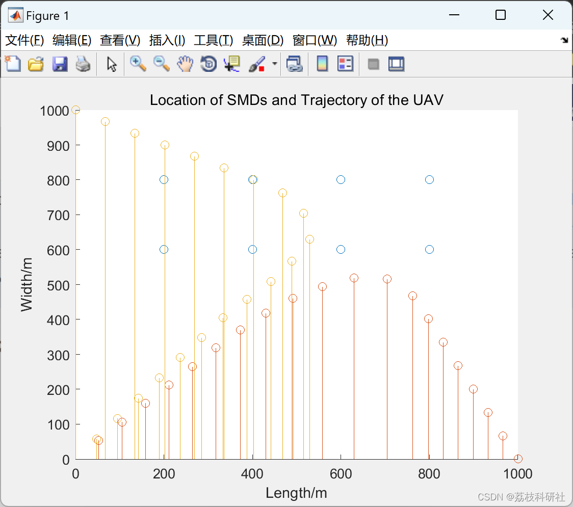
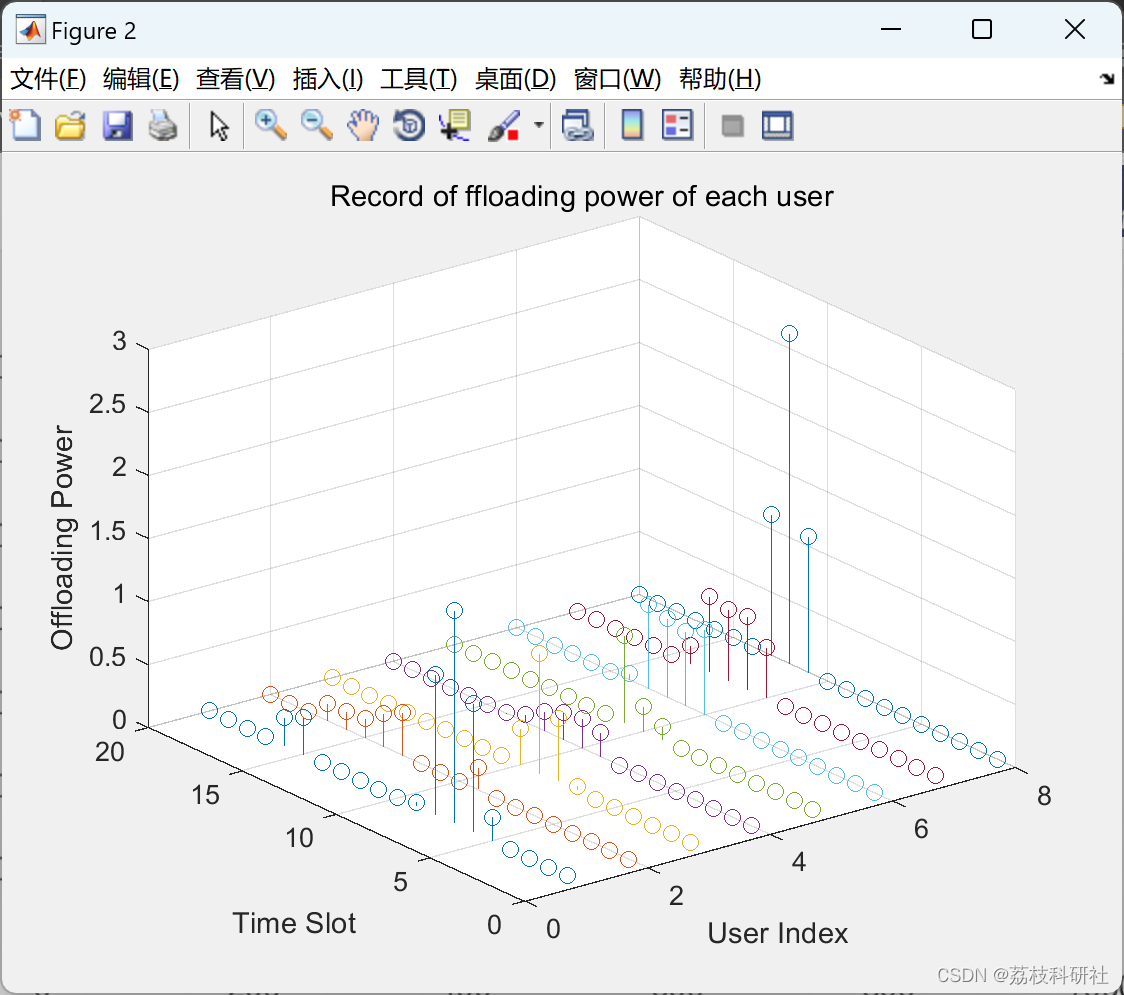
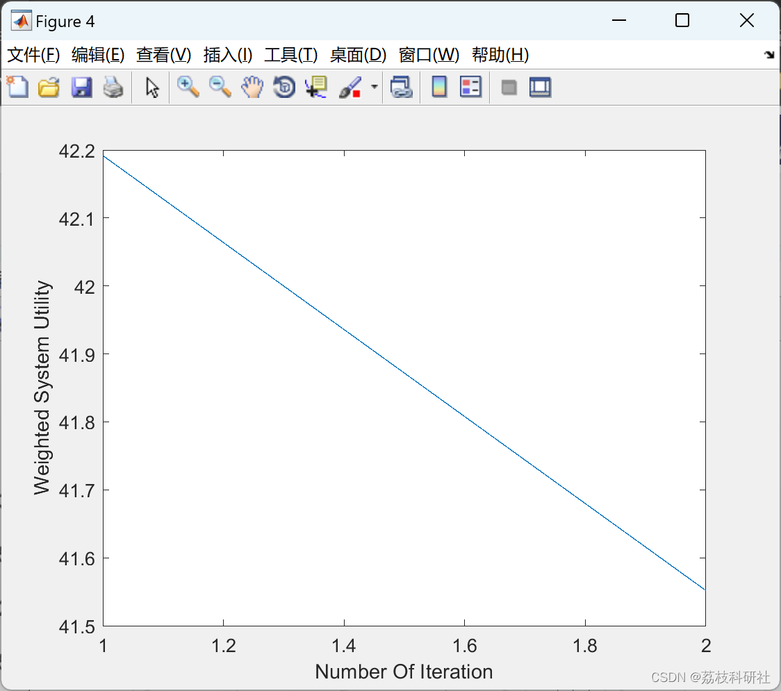
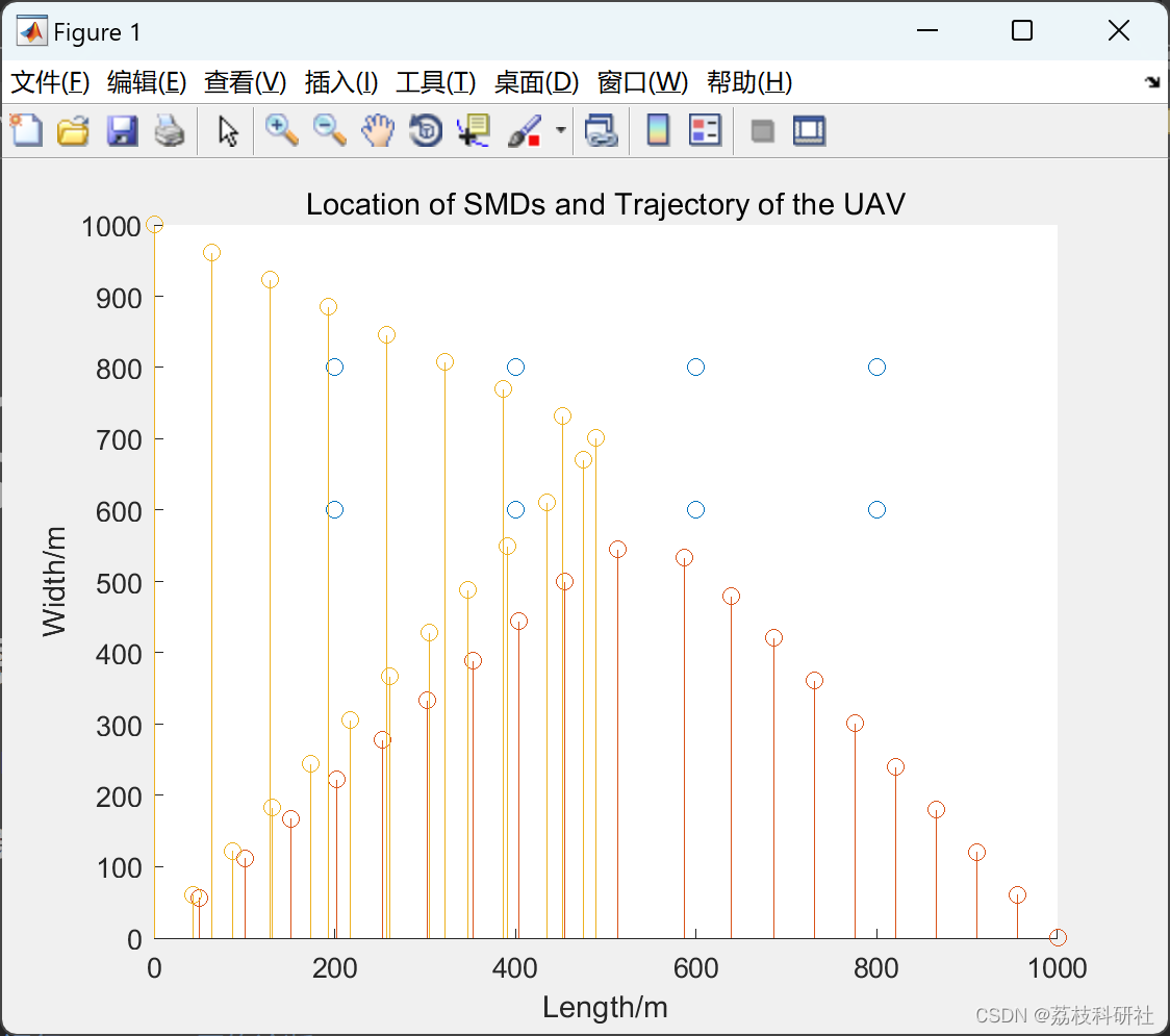
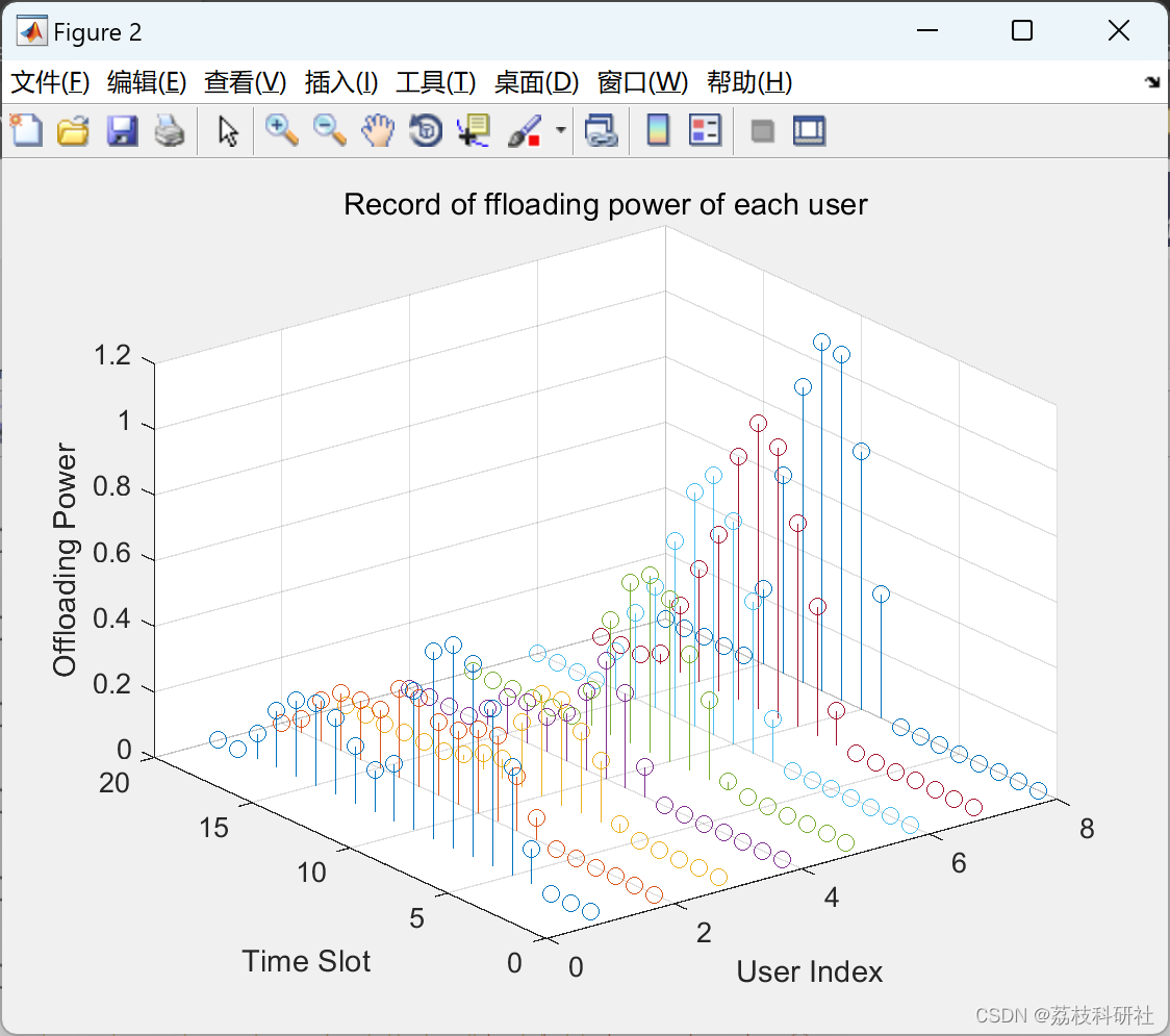
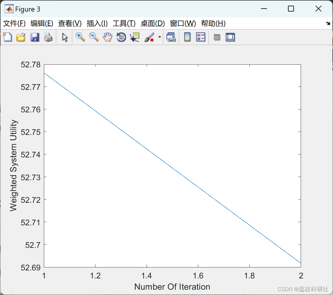
摘要：多接入边缘计算（MEC）被认为是克服移动设备计算能力限制的有前途的解决方案。本文研究了一种基于非正交多址（NOMA）的节能无人机MEC框架，将多架无人机部署为边缘服务器，为地面用户提供计算辅助，并采用NOMA降低任务卸载能耗。形成一个实用程序以数学方式评估系统的加权能源成本。由于参数的耦合，效用最小化是一个高度非凸的问题，因此，该问题被分解为两个更易于处理的子问题，即给定无人机轨迹的无线电和计算资源的最优分配，以及基于给定资源分配方案的轨迹规划。这两个问题分别通过逐次凸逼近（SCA）和二次逼近转换为凸问题。然后，提出一种高效的迭代算法，交替求解这两个子问题，逐步接近所提系统的最优资源管理。大量的数值结果表明，所提出的策略在能源效率方面比现有系统具有显著优势。

原文摘要：

Abstract:

Multiaccess edge computing (MEC) is regarded as a promising solution to overcome the limit on the computation capacity of mobile devices. This article investigates an energy-efficient unmanned aerial vehicle (UAV)-enabled MEC framework incorporating nonorthogonal multiple access (NOMA), where multiple UAVs are deployed as edge servers to provide computation assistance to terrestrial users and NOMA is adopted to reduce the energy consumption of task offloading. A utility is formed to mathematically evaluate the weighted energy cost of the system. Due to the coupling of parameters, the minimization of utility is a highly nonconvex problem and therefore, the problem is decomposed into two more tractable subproblems, i.e., the optimal allocation of radio and computation resources given UAV trajectories, and the trajectory planning based on given resource allocation schemes. These two problems are converted to convex ones via successive convex approximation (SCA) and quadratic approximation, respectively. Then, an efficient iterative algorithm is proposed where these two subproblems are alternately solved to gradually approach the optimal resource management of the proposed system. Sufficient numerical results show that our proposed strategy has a remarkable advantage over existing systems in terms of energy efficiency.

📚2 运行结果

 

 

 

 

 

部分代码：

% This script describes a NOMA-assisted MEC system on UAV according to doc 'Model 1.pages'.
% Created and copyrighted by ZHANG Xiaochen at 10:22 a.m., Apr. 12, 2019.

%% Setup of the Model

% Consider U terrestrial users located in a area
U = 8;                                                 % Number of users/SMDs

% The size of the area is defined by:
lengthArea = 1000;                            % Length of the coverage area (m)
widthArea = 1000;                             % Width of the coverage area (m)

% U SMDs are uniformly distributed in the rectangular coverage area.
rUser = [lengthArea*rand(U, 1),widthArea*rand(U, 1), zeros(U, 1)];
% rUser = [100*(2:2:8).', 100*8*ones(U, 1), zeros(U, 1)];
% rUser = [[400,400,600,600].', [600,800,600,800].',zeros(U, 1)];
% rUser = [[100,500,800,600].', [600,600,600,800].',zeros(U, 1)];
rUser = [kron(100*(2:2:8).',ones(2,1)), ...
    repmat([600, 800].', 4, 1),...
    zeros(U, 1)];

% Divide the time interval into N tme slots.
T = 100;                                               % Length of interval
N = 20;                                                 % Number of time slots
tau = T/N;                                            % Duration of each time slot

% Set the initial trajectory of UAV
M = 2;
hUAV = 50;                                         % Flying altitude of UAV
rI = [0, 0, hUAV; 0, 0, hUAV];              % Intial position of the UAV (M*3)
rF = [lengthArea, 0, hUAV; 0, widthArea, hUAV];               % Final position of the UAV

rUAV = zeros(N, 3, M);                             % Trajectory vector of the UAV

% rUAV(time, dimension, UAV index) is a N*3*M matrix of which each describes the 3-D coordinates of UAVs
% at each time slot.

for m = 1:M
    rUAV(N, :, m) = rF(m, :);
end
for n = 1:N-1
    for m = 1:M
        rUAV(n, :, m) = rI(m, :)+n/N*(rF(m, :)-rI(m, :));
    end
end

% Other parameters involved in the model.

omegaUser = 0.8;                        % Weight factor of users
omegaUAV = 1-omegaUser;         % Weight factor of UAVs

N0 = 1e-17;                                 % Power spectral density of AWGN (W/Hz)
B = 4e6;                                        % System bandwidth (Hz)

D = 120*ones(U, 1);                     % Number of bits for each SMDs to finish (Mbit)
kappa = 1e-28;                            % Effective swiched capacitance of CPU

fmaxUAV = 20;                            % Maximum CPU frequency of MEC server (GHz)
fminUAV = 0;                               % Minimum CPU frequency of SMDs (GHz)
CUAV = 1e3;                                % Processing density of MEC server (Hz/bit)

🎉3 参考文献

部分理论来源于网络，如有侵权请联系删除。

🌈4 Matlab代码实现