


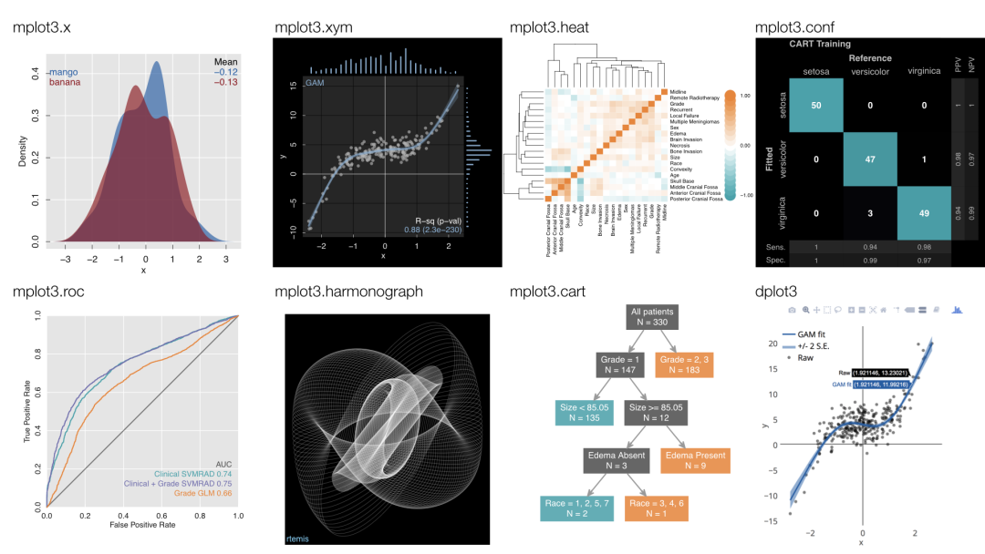
rtemis 是一个集机器学习与可视化于一体的 R 包,用于各种高级机器学习研究和应用。整体而言,该软件有三个目标:
-
「应用数据科学」:使高级数据分析高效且易于使用
-
「机器学习研究」:提供一个平台以开发和测试新颖的机器学习算法
-
「教育」:通过提供简明的案例、代码和可视化,使机器学习概念易于理解
比较有特点的是,rtemis 为数据处理、监督学习和聚类提供了大量算法的通用函数接口。小编在官网中看到的包装功能确实也多:
-
预处理
-
保持完整样本:可以选择仅保留没有缺失数据的样本。
-
移除常量特征:删除所有值都相同的列。
-
移除重复样本:删除重复的行。
-
根据缺失数据比例移除样本或特征:根据缺失数据的阈值删除样本或特征。
-
数据类型转换:将整数、逻辑值和字符变量转换为因子、数字或其他类型。
-
数值变量的分箱:将数值变量根据区间或分位数进行分箱处理。
-
处理缺失值:生成指示缺失数据的新布尔列,并选择多种方法进行缺失值插补。
-
数据缩放和中心化:对列进行标准化处理。
-
独热编码:将因子变量进行独热编码。
-
-
重采样
-
bootstrap:标准自助法,即带放回的随机抽样。
-
strat.sub:分层样本抽样。
-
strat.boot:先进行分层子样本抽样,然后随机复制一些训练样本以达到原始长度或指定长度。
-
kfold:k折交叉验证。
-
loocv:留一交叉验证。
-
-
无监督学习
-
聚类
-
分解 / 降维
-
-
监督学习
-
回归与分类
-
自动调参与测试
-
实验记录
-
集成法
-
提升法
-
RuleFit 算法
-
类别不平衡数据的处理
-
集成模型
-
叠加树模型
-
线性叠加树模型
-
在本文中,仅仅展示如何使用 rtemis 快速进行分类与回归,更多个性化的内容大家可以参照下方的「官方文档」:
-
https://rtemis.lambdamd.org/
0. R包下载
用户可以通过以下代码安装或者引用:
# 从GitHub上安装该包
remotes::install_github("egenn/rtemis")
# 其它潜在的依赖包
install.packages("mlbench")
install.packages("pROC")
install.packages("PRROC")
install.packages("progressr")
install.packages("future.apply")
1. 回归模型
① 生成用于回归的模拟数据框dat:
x <- rnormmat(500, 5, seed = 2019)
y <- x %*% rnorm(5) + rnorm(500)
dat <- data.frame(x, y)

# check 函数用于检查数据集的整体概况
check_data(dat)
#  dat: A data.table with 500 rows and 6 columns
#  Data types
#  * 6 numeric features
#  * 0 integer features
#  * 0 factors
#  * 0 character features
#  * 0 date features

#  Issues
#  * 0 constant features
#  * 0 duplicate cases
#  * 0 missing values

#  Recommendations
#  * Everything looks good

# 最后简单看一下dat
head(dat)
#          X1         X2          X3         X4         X5          y
#1  0.7385227 -0.5201603  1.63030574  1.9567386 -0.7911291  3.9721257
#2 -0.5147605  0.5388431  0.47104282  0.8373285  0.8610578 -1.7725552
#3 -1.6401813  0.2251481 -0.73062473 -0.6192940  1.1604909 -3.3698612
#4  0.9160368 -1.5559318 -0.05606844  0.4602711 -0.9290626  5.1083103
#5 -1.2674820 -0.2355507  0.71840950 -0.9094905 -1.1453902 -2.8096872
#6  0.7382478  1.1090225  0.80076099  1.1155501  1.5148726 -0.3089569
dat的行代表样本,列X1-X5分别代表不同的特征变量,列y代表用于回归的目标变量(因变量)。同样的,对于自己的数据也是按照类似的格式准备。
② 重新采样,生成训练集与测试集列表res:
res <- resample(dat,
                resampler = "strat.sub", # 选用分层抽样。
                stratify.var = y,        # 用于分层的指定变量
                strat.n.bins = 4,       # 将分层变量划分为3个区间,确保每个区间的数据在训练集和测试集中都能存在,使得测试集的结果更为可信
                train.p = 0.75,         # 每层中随机选取75%的样本作为新的数据集
                n.resamples = 10        # 需要生成的重采样数据集数量
                )
这里使用的是默认参数resampler = "strat.sub"进行分层抽样,其原理根据指定的分层变量(stratify.var参数,这里是y)将数据集分成多个组(层),在每个层内按照指定的比例(train.p=0.75)随机抽取样本,产生新的队列。n.resamples设置为10,意味着将分别抽样10次,总共生成10个新的队列,并以列表res返回抽样对列的行索引。
# 简单看一下res,每个Subsample_*对应不同的索引,可以用于提取指定的抽样数据集
str(res)
#List of 10
# $ Subsample_1 : int [1:374] 1 4 6 8 9 12 14 17 18 19 ...
# $ Subsample_2 : int [1:374] 2 3 4 5 6 8 10 11 14 15 ...
# $ Subsample_3 : int [1:374] 1 2 3 4 6 8 9 10 11 13 ...
# $ Subsample_4 : int [1:374] 1 3 4 5 6 7 8 12 14 15 ...
# $ Subsample_5 : int [1:374] 2 4 5 6 8 10 12 14 15 16 ...
# $ Subsample_6 : int [1:374] 1 2 3 4 5 6 7 8 9 10 ...
# $ Subsample_7 : int [1:374] 3 4 5 6 7 8 10 11 12 14 ...
# $ Subsample_8 : int [1:374] 1 2 3 5 6 7 8 10 11 13 ...
# $ Subsample_9 : int [1:374] 1 2 3 4 5 6 7 8 9 10 ...
# $ Subsample_10: int [1:374] 1 2 4 5 6 7 8 10 11 12 ...
# - attr(*, "class")= chr [1:2] "resample" "list"
# - attr(*, "N")= int 10
# - attr(*, "resampler")= chr "strat.sub"
# - attr(*, "train.p")= num 0.75
# - attr(*, "strat.n.bins")= num 4
③ 指定训练集与测试集并构建模型
# 训练集为分层采样后的第一个数据集
dat.train <- dat[res$Subsample_1, ]
# 第一个数据集分层采样剩下的数据集作为测试集
dat.test <- dat[-res$Subsample_1, ]
# 构建模型
mod <- s_GLM(dat.train, dat.test)
mod$describe()
#Generalized Linear Model was used for regression.
#R-squared was 0.98 (training).

# 简单看一下常见的几个回归指标
mod$error.train      # 训练集
#MSE = 1.02 (97.81%)
#RMSE = 1.01 (85.18%)
#MAE = 0.81 (84.62%)
#r = 0.99 (p = 1.3e-310)
#R sq = 0.98
mod$error.test      # 测试集
#MSE = 0.98 (97.85%)
#RMSE = 0.99 (85.35%)
#MAE = 0.76 (85.57%)
#r = 0.99 (p = 2.7e-105)
#R sq = 0.98

# 测试集上的预测结果,训练集的预测结果可以通过mod$fitted打印
mod$predicted
#  [1]  -6.9228634  13.5473120  -4.4142316  -6.4150050  -3.1899404   5.8635544  10.9276092  -3.3697528   7.3197323   4.5917325   3.8279902
# [12]  -2.5436844  -8.4399966  -3.2597535   3.0558347  10.1805533  -4.5057564  -0.1087756  -0.7984958  -8.4851937  -4.8099938  -0.7611819
# [23]  -0.3023645  -1.1838060   6.2697071   2.9259362   2.9894219   3.5715647   3.2065868   2.3246177  -1.1029005  -3.1490491  -7.2180310
# [34]   1.3552666   8.1584272  -2.2085630  -1.5803727  -0.7588147   1.4364268   0.6639963   5.3642140   0.3600681  -4.2238833 -18.8447897
# [45]  -6.2053170  -5.6646543  -6.3526682   5.9058403  -2.9385554  -1.8897201   3.3465618   3.1953050   1.9692337  -8.0531435   0.4722245
# [56]  14.6760641  -1.6578528  11.2129667  -9.2015635   0.6143482  -2.8688158  -1.5580413   0.3452240 -19.3633269  -4.7365043  -1.7222169
# [67]  -3.5001696   2.0906088  -5.5367285  16.0566618  -2.2632949  10.1779890   4.8057160   5.0095983  -3.4675440  -7.8418409   1.5149870
# [78]  -1.0510093   1.2397077   7.8981605   0.1196208 -13.6210350  -2.1589314  -4.5641406  -4.9111480  -0.5444266   3.8954173 -15.3977663
# [89]  -6.3044076  -5.8120357   0.2301799  -1.8128115   4.7353047 -11.5507244   2.2981759 -11.6778343  -4.4418715   4.5915911  13.0456691
#[100]   2.3961443  11.6771535   2.9362587   3.4500863  14.6597287   7.2120194  -6.8395880 -17.1198556   8.7869138  -3.8199982  -5.0879467
#[111]  -3.9051859  -9.9320098   0.5141523  -6.2265527  -6.1502030  10.6211752  -1.2735560   3.0118796   3.2969205  -1.8482288   3.6860180
#[122]   0.6108124  10.0208633   5.8474645   1.4720176   0.2498226
需要注意,构建回归模型的函数s_GLM默认使用最后一列作为因变量/目标变量(其实这个函数参数超级多,感兴趣的铁子可以自行学习指定)。同时,s_GLM 既支持 线性回归 和 逻辑回归(单分类任务),也支持 多项逻辑回归(也就是多分类任务)。对于多分类任务,如果 y 有两个以上的类别,s_GLM内部使用nnet::multinom进行多项逻辑回归。
④ 可视化模型结果:
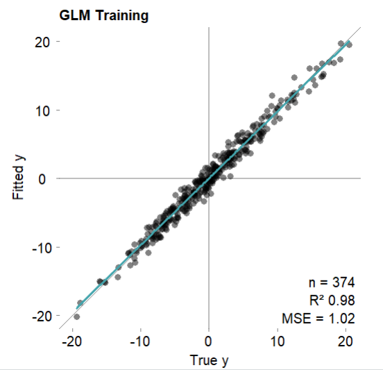
# 可视化训练集拟合结果
mod$plotFitted(theme = 'white')
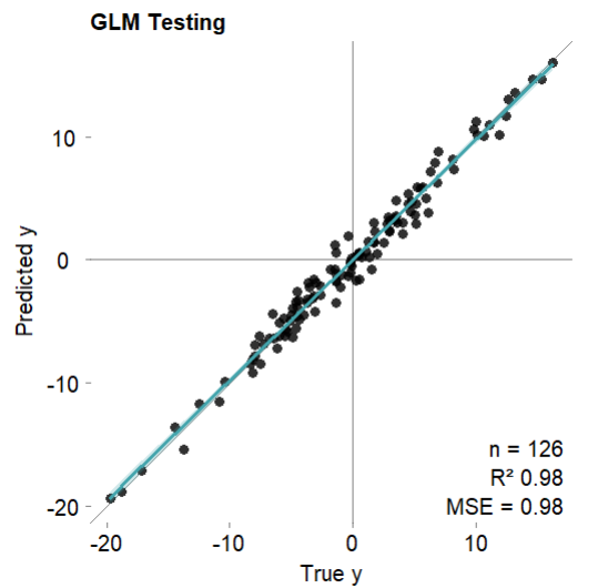
# 可视化测试集拟合结果
mod$plotPredicted(theme = 'white')
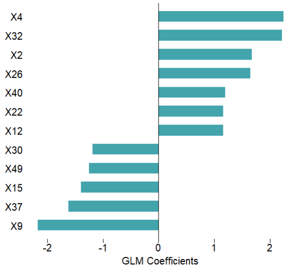
# 可视化特征重要性
mod$plotVarImp(theme = 'white')
需要注意,返回的mod是 R6 类对象。R6 对象包含属性和函数,同时支持 S3 方法,因此用户可以访问所有熟悉的 R 泛型。
2. 分类模型
① 示例数据的准备,这里使用的是mlbench的内置数据集,总共有 60 个特征与最后一列的 Class 的分类属性:
data(Sonar, package = 'mlbench')
str(Sonar)
#'data.frame': 208 obs. of  61 variables:
# $ V1   : num  0.02 0.0453 0.0262 0.01 0.0762 0.0286 0.0317 0.0519 0.0223 0.0164 ...
# $ V2   : num  0.0371 0.0523 0.0582 0.0171 0.0666 0.0453 0.0956 0.0548 0.0375 0.0173 ...
# $ V3   : num  0.0428 0.0843 0.1099 0.0623 0.0481 ...
# $ V4   : num  0.0207 0.0689 0.1083 0.0205 0.0394 ...
# $ V5   : num  0.0954 0.1183 0.0974 0.0205 0.059 ...
# $ V6   : num  0.0986 0.2583 0.228 0.0368 0.0649 ...
# $** .........................................
# $ V60  : num  0.0032 0.0044 0.0078 0.0117 0.0094 0.0062 0.0103 0.0053 0.0022 0.004 ...
# $ Class: Factor w/ 2 levels "M","R": 2 2 2 2 2 2 2 2 2 2 ...

# 检查一下数据
check_data(Sonar)
#  Sonar: A data.table with 208 rows and 61 columns
#  Data types
#  * 60 numeric features
#  * 0 integer features
#  * 1 factor, which is not ordered
#  * 0 character features
#  * 0 date features
#  Issues
#  * 0 constant features
#  * 0 duplicate cases
#  * 0 missing values
#  Recommendations
#  * Everything looks good
② 数据重采样分组(与上面回归模型的一致):
res <- resample(Sonar)
sonar.train <- Sonar[res$Subsample_1, ]
sonar.test <- Sonar[-res$Subsample_1, ]
③ 模型的构建,s_Ranger函数是该包提供的用于构建随机森林的分类/回归模型,内部提供了多种参数(包括常见的mtry,用于自动调参的autotune等等)
mod <- s_Ranger(sonar.train, sonar.test)
# 简答看看模型的描述
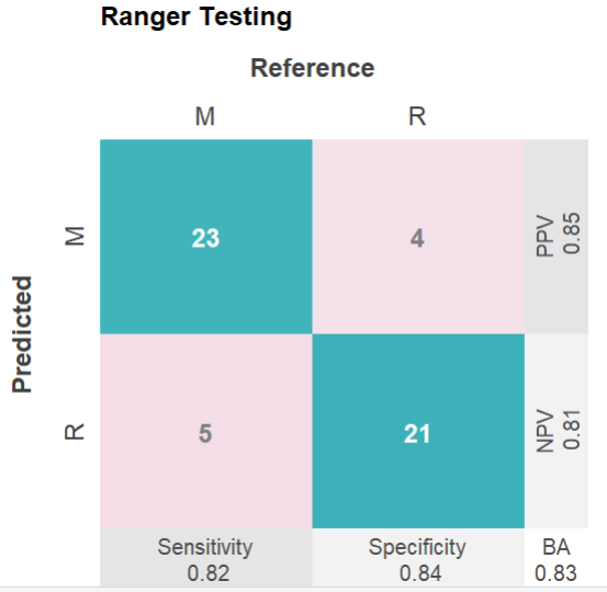
mod$describe()
#Ranger Random Forest was used for classification.
#Balanced accuracy was 1 (training)and 0.83 (testing).
④ 可视化结果(基本上训练集测试集都有,命名也是具有统一规律,这边就只展示其中一张)
mod$plotPredicted(theme = 'white') # 测试集,分类性能的四格热图
mod$plotFitted(theme = 'white')    # 训练集
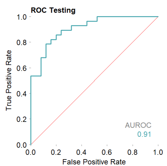
mod$plotROCpredicted(theme = 'white')# 测试集,分类性能的roc曲线
mod$plotROCfitted(theme = 'white')   # 训练集
mod$plotPRpredicted(theme = 'white')# 测试集,分类性能的PR曲线
mod$plotPRfitted(theme = 'white')   # 训练集

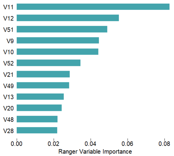
mod$plotVarImp(theme = 'white')# 特征重要性
三. 可视化主题
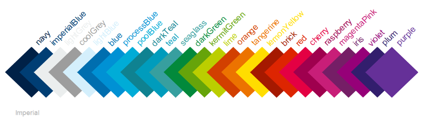
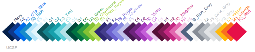
① 配色系列,rtpalette函数提供了多种可供选择的配色系列:
rtpalette()
#[1] "ucsfCol"             "pennCol"             "imperialCol"         "stanfordCol"         "ucdCol"
#[6] "berkeleyCol"         "ucscCol"             "ucmercedCol"         "ucsbCol"             "uclaCol"
#[11] "ucrColor"            "uciCol"              "ucsdCol"             "californiaCol"       "scrippsCol"
#[16] "caltechCol"          "cmuCol"              "princetonCol"        "columbiaCol"         "yaleCol"
#[21] "brownCol"            "cornellCol"          "hmsCol"              "dartmouthCol"        "usfCol"
#[26] "uwCol"               "jhuCol"              "nyuCol"              "washuCol"            "chicagoCol"
#[31] "pennstateCol"        "msuCol"              "michiganCol"         "iowaCol"             "texasCol"
#[36] "techCol"             "jeffersonCol"        "hawaiiCol"           "nihCol"              "torontoCol"
#[41] "mcgillCol"           "uclCol"              "oxfordCol"           "nhsCol"              "ethCol"
#[46] "rwthCol"             "firefoxCol"          "mozillaCol"          "appleCol"            "googleCol"
#[51] "amazonCol"           "microsoftCol"        "pantoneBalancingAct" "pantoneWellspring"   "pantoneAmusements"
#[56] "grays"               "rtCol1"              "rtCol3"
简单给各位铁子看看:
previewcolor(rtpalette("imperialCol"), "Imperial", bg = "white")
previewcolor(rtpalette("ucsfCol"), "UCSF", bg = "white")
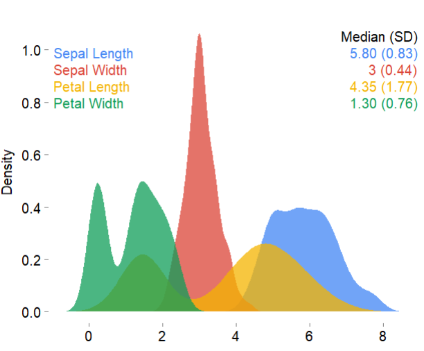
具体使用的时候可以指定参数palette:
mplot3_x(iris, palette = "google", theme = 'white')
② 主题,可选的主题包括以下几种:
-
white
-
whitegrid
-
whiteigrid
-
black
-
blackgrid
-
blackigrid
-
darkgray
-
darkgraygrid
-
darkgrayigrid
-
lightgraygrid
-
mediumgraygrid
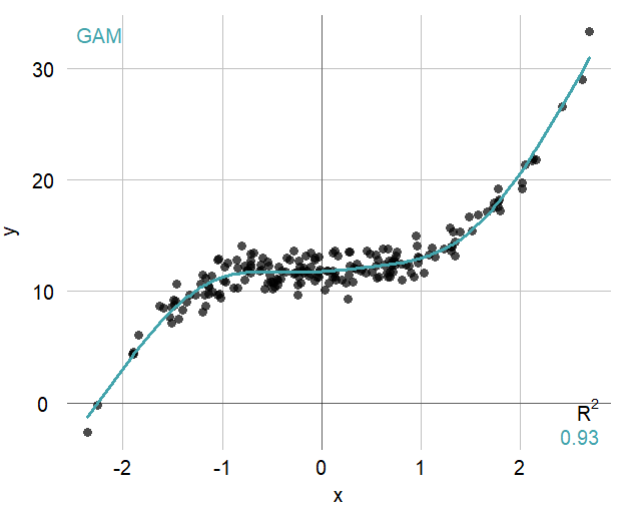
具体使用的时候指定theme参数即可:
set.seed = 2019
x <- rnorm(200)
y <- x^3 + 12 + rnorm(200)
mplot3_xy(x, y, theme = 'whitegrid', fit = 'gam')
传统的机器学习 R 包确实不少
但今天分享的有一些特点
首先是大量可供选择的算法
封装的不错,参数很多
简便易行
其次是提供建模前的预处理方法
最后是兼顾数据可视化
就分享到这


 1万+
1万+


 被折叠的 条评论
为什么被折叠?
被折叠的 条评论
为什么被折叠?
 到【灌水乐园】发言


