


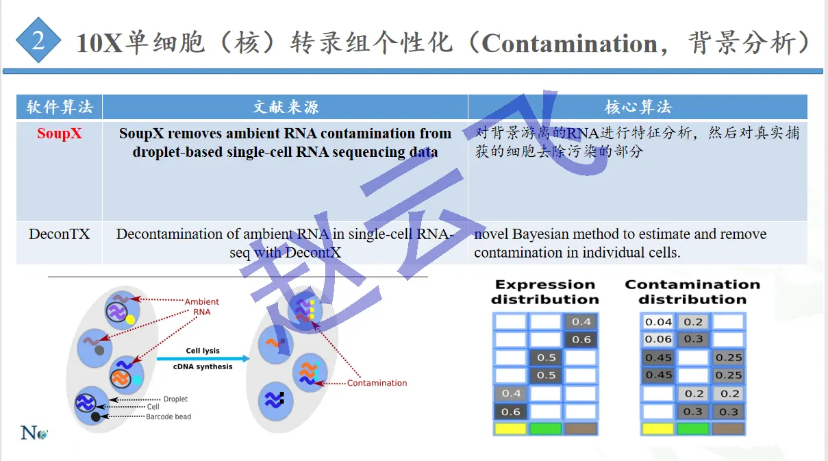
hello,大家好,今天给大家带来一个10X空间转录组去除污染的方法,具体怎么做,大家往下看,文章在SpotClean adjusts for spot swapping in spatial transcriptomics data其实关于去除污染的方法,很多都是针对单细胞数据游离污染的,大家可以参考我之前讲的公开课。
好了,我们来看看10X空间转录组的污染以及如何去除。
summary
空间转录组学 (ST) 是一种强大且广泛使用的方法,用于分析组织中的全基因组基因表达,在分子医学和肿瘤诊断中具有新兴应用。 最近的空间转录组学实验利用包含数千个点的载玻片,这些点具有结合 mRNA 的点特异性条形码。 理想情况下,一个点的唯一分子标识符测量点特定的表达,但由于附近点的bleed,这通常不是这种理想情况,可以将其称为点交换。 所以建议使用SpotClean调整spot swapping ,并在此过程中提高进行下游分析的灵敏度和精度。 (也就是说空间转录组的污染主要来自于周周围spot mRNA的游离)。
简介
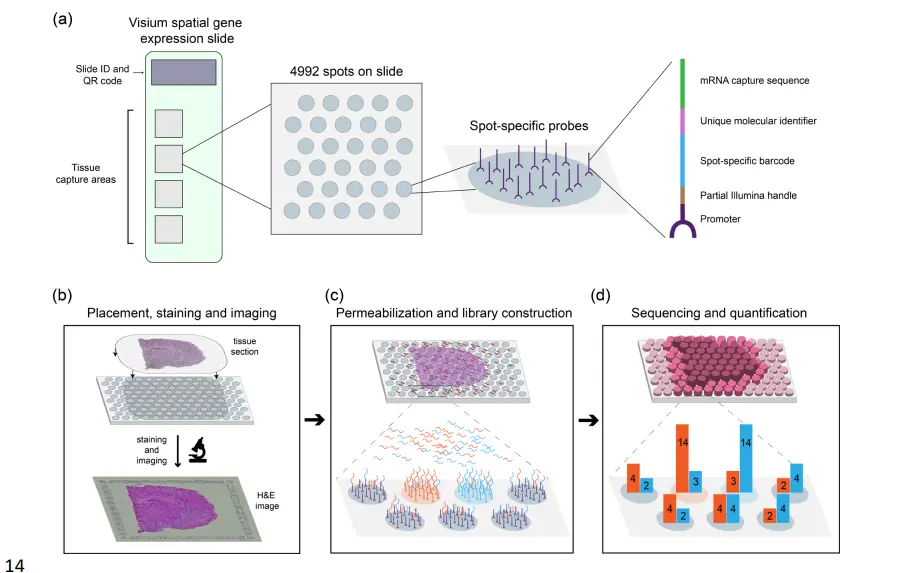
在典型的 ST 实验中,将新鲜冷冻(或 FFPE)组织切片并放置在含有spot的载玻片上,每个spot包含数百万个具有该spot独特空间条形码的捕获寡核苷酸。组织成像,通常通过苏木精和伊红 (H&E) 染色。成像后,组织被透化以释放 mRNA,然后与捕获寡核苷酸结合,生成一个 cDNA 文库,该文库由保留空间信息的条形码结合的转录本组成。 ST 实验的数据由组织图像和从每个点收集的 RNA 测序数据组成。处理 ST 数据的第一步是组织检测,其中包含组织的载玻片上的点与没有组织的背景点区分开来。然后在包含组织的每个点上的唯一分子标识符 (UMI) 计数用于下游分析 (下图)。
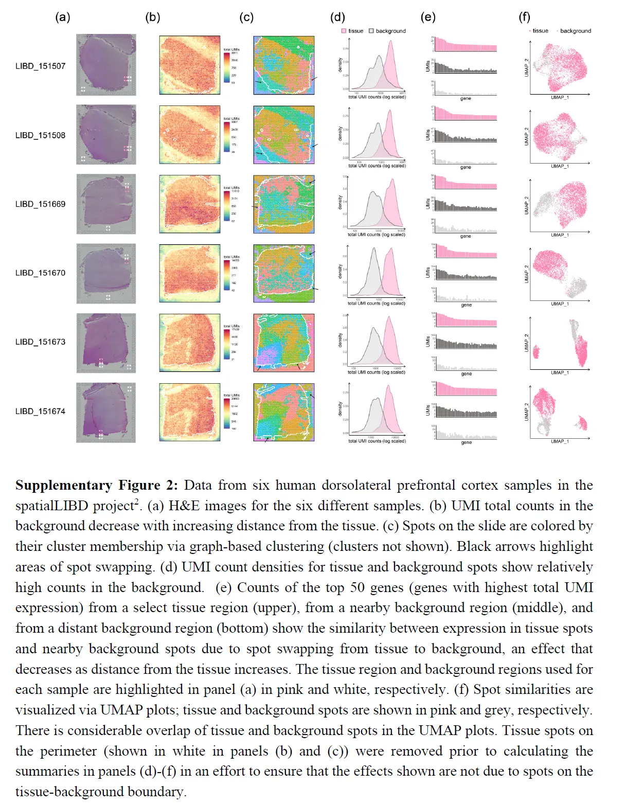
理想情况下,给定spot的基因特异性 UMI 将代表该基因在该点的表达,而没有组织的spot将不显示 UMI。实际情况并非如此。从附近spot流出的信使 RNA 会导致 UMI 计数的大量污染,这里将这种现象称为点交换。下图显示了死后人类大脑组织样本中的点交换证据,该组织样本被描述为空间 LIBD 的一部分,该项目旨在定义六层人类背外侧前额叶皮层 (DLPFC) 中基因表达的。
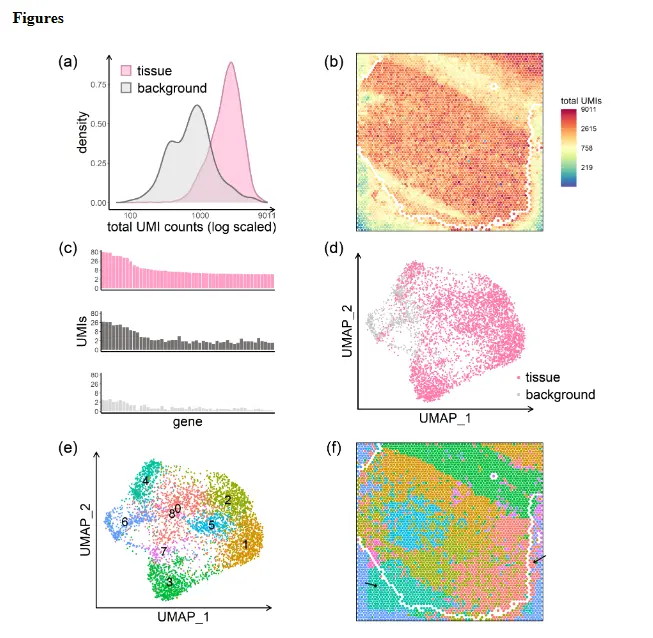
- 注: Data from the human dorsolateral prefrontal cortex profiled in the spatialLIBD experiment,sample LIBD_151507. (a) UMI count densities for tissue and background spots show relatively high counts in the background. (b) UMI total counts in the background decrease with increasing distance from the tissue;the perimeter delineating tissue and background is shown in white. (c) Counts of the top 50 genes from a select tissue region (upper), from a nearby background region (middle), and from a distant background region (bottom) show the similarity between expression in tissue spots and nearby background spots due to spot swapping from tissue to background, an effect that decreases as distance from the tissue increases. (d) Tissue and background spots are not distinguished visually via UMAP. (e) Graph-based clustering of all spots identifies 9 clusters. (f) Spots on the slide are colored by their cluster membership shown in (e). Black arrows highlight areas of spot swapping of signal from tissue to background. Spots on the perimeter (shown in white) have been removed from the summaries shown here to ensure that the effects shown are not due to spots on the tissue-background boundary.
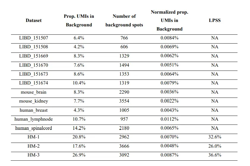
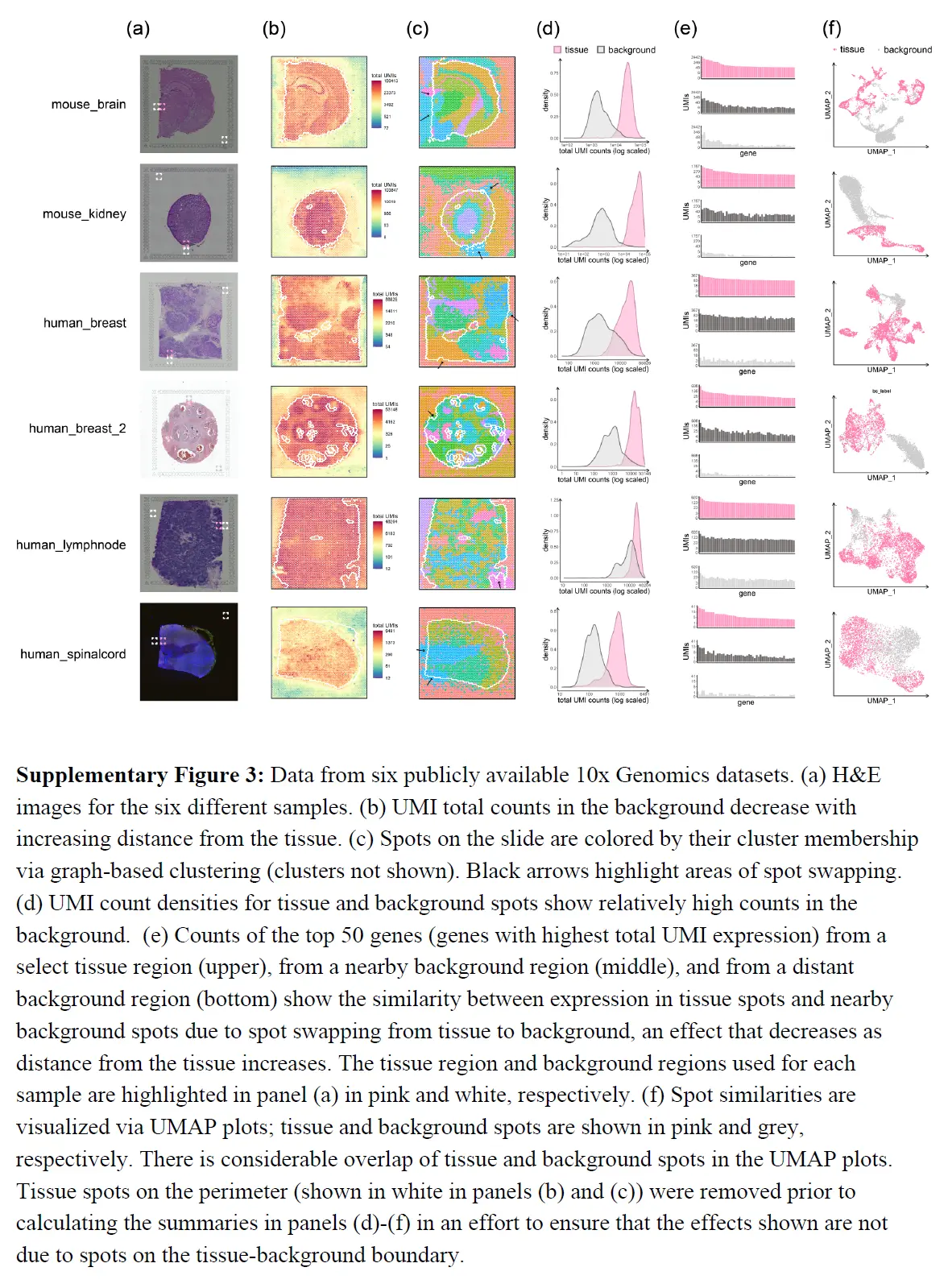
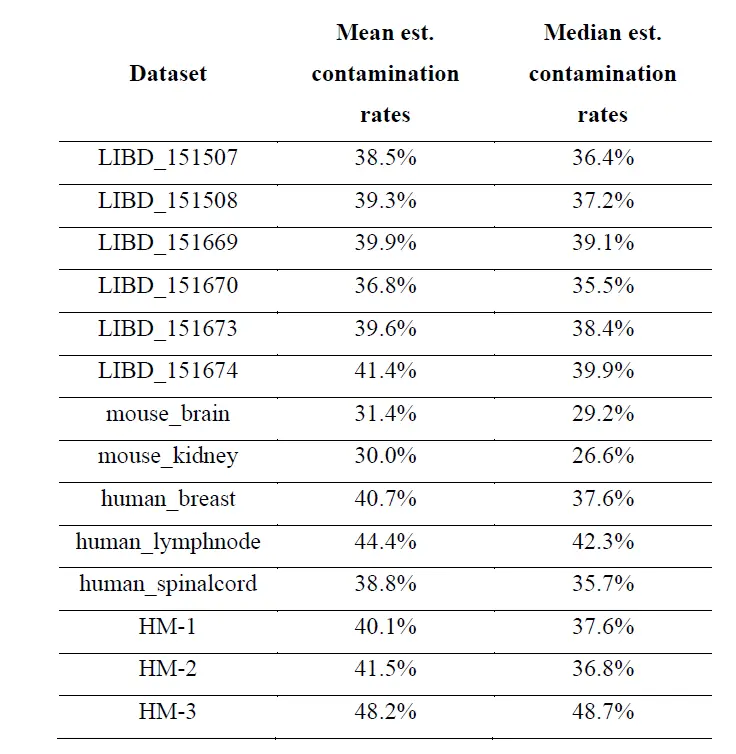
具体来说,上图a 显示背景点的 UMI 计数(在没有污染的情况下为零)与组织点的计数相比较高;并且计数随着与组织距离的增加而减少(上图b)。上图c 显示了组织区域、附近背景区域和远处背景区域中 50 个基因的 UMI 计数分布。由于组织和附近背景之间的表达相似性,组织和背景斑点不容易区分(上图d)。这在上图f 中再次得到强调,where spots on the slide are 46 colored by membership in the graph-based clusters shown in 上图e。其他数据的测试显示了类似结果;下表显示,在大多数数据集中,背景点中 UMI 计数的比例在 5% 到 20% 之间。
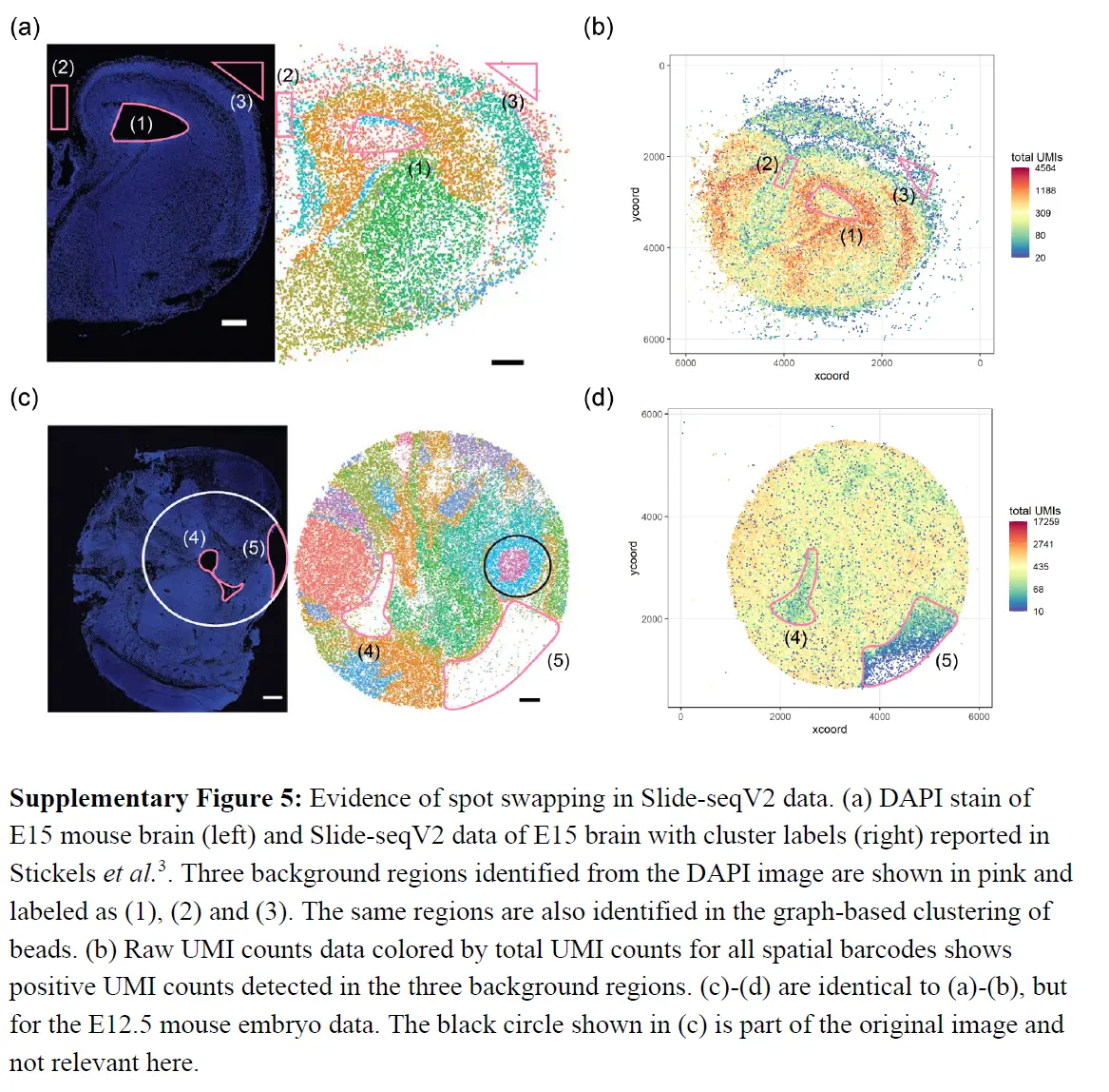
下面又是一些证明的例子
上面的结果表明从组织到背景发生点交换,但评估从组织spot到组织spot的点交换程度更具挑战性。虽然 SpotClean 模型提供了一个估计值(下表),
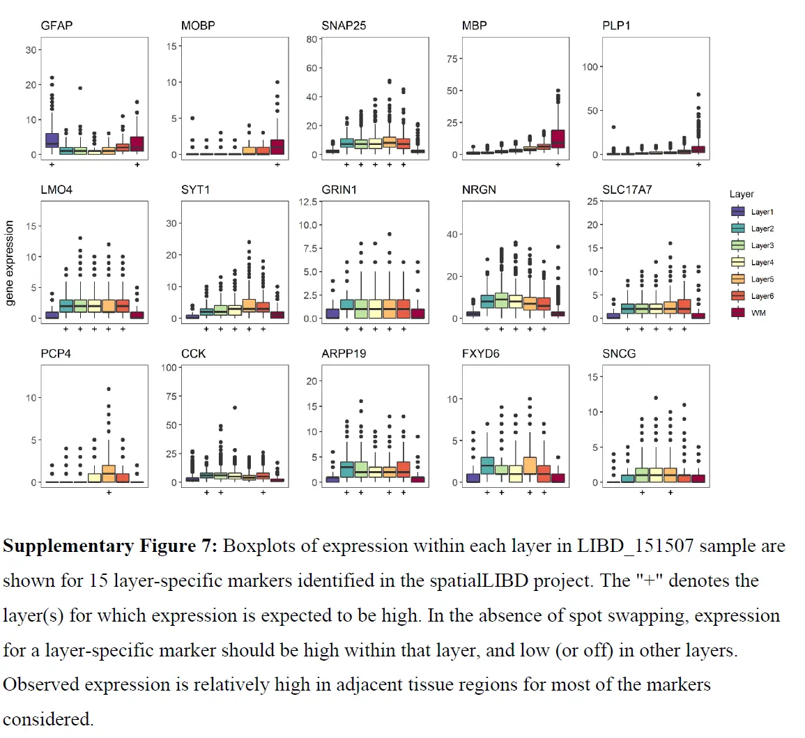
但也考虑了在 spatialLIBD 项目中识别的组织特异性标记基因。在没有点交换的情况下,层特定标记的表达在该层中应该很高,而在其他层中应该很低(或关闭)。当点交换发生时,附近层中的标记表达相对较高。这在 GFAP 中很明显,例如,一种已知在白质 (WM) 和 DLPFC 的第一个注释层 (Layer1) 中上调的标记。下图显示了 GFAP 在 WM 和 Layer1 斑点中的高表达,
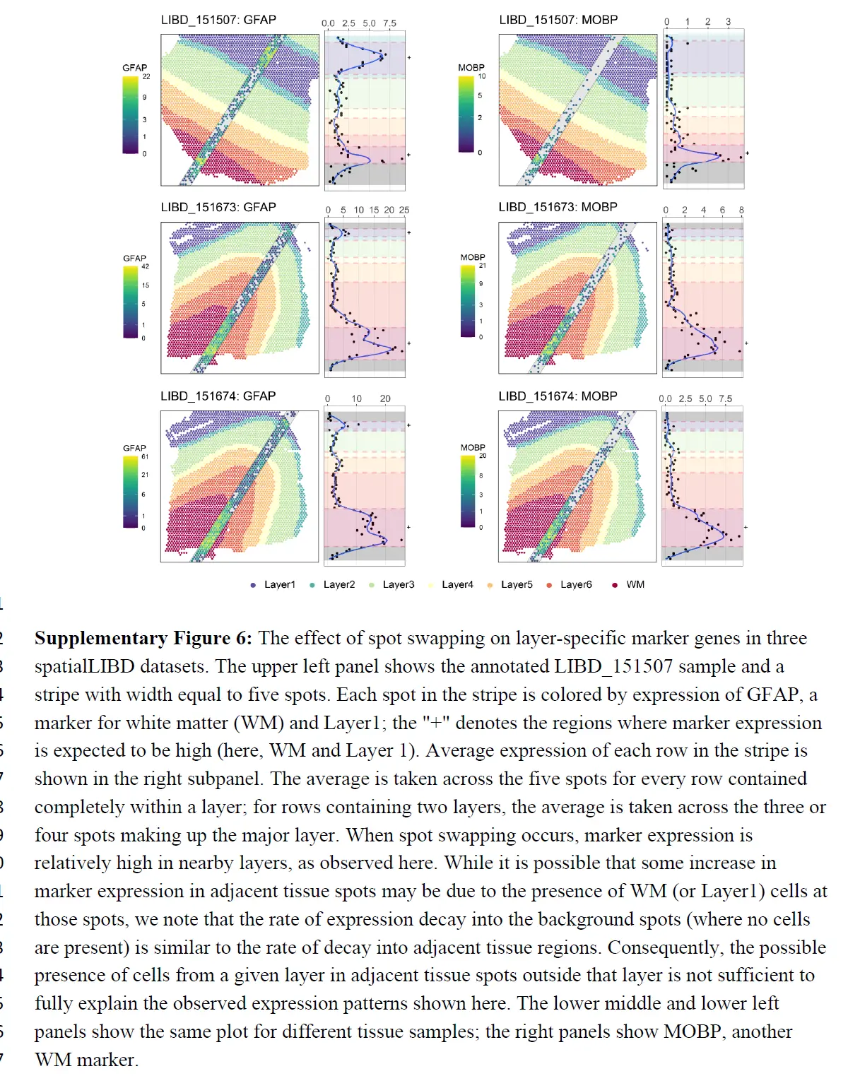
正如预期的那样,但在与 WM 和 Layer1 相邻的组织spot中也有相对高的表达,GFAP 表达随着与 WM(或 Layer1)的距离增加而降低。虽然相邻组织spot中标记物表达的一些增加可能是由于这些斑点处存在 WM(或 Layer1)细胞,但应该注意到表达速率衰减到背景斑点(其中不存在细胞)类似于衰减到相邻组织区域的速率。因此,相邻组织斑点中可能存在的 WM(或 Layer1)细胞不足以完全解释观察到的表达模式。 WM 标记、MOBP(上图)以及 13 个附加标记(下图)显示了类似的结果。
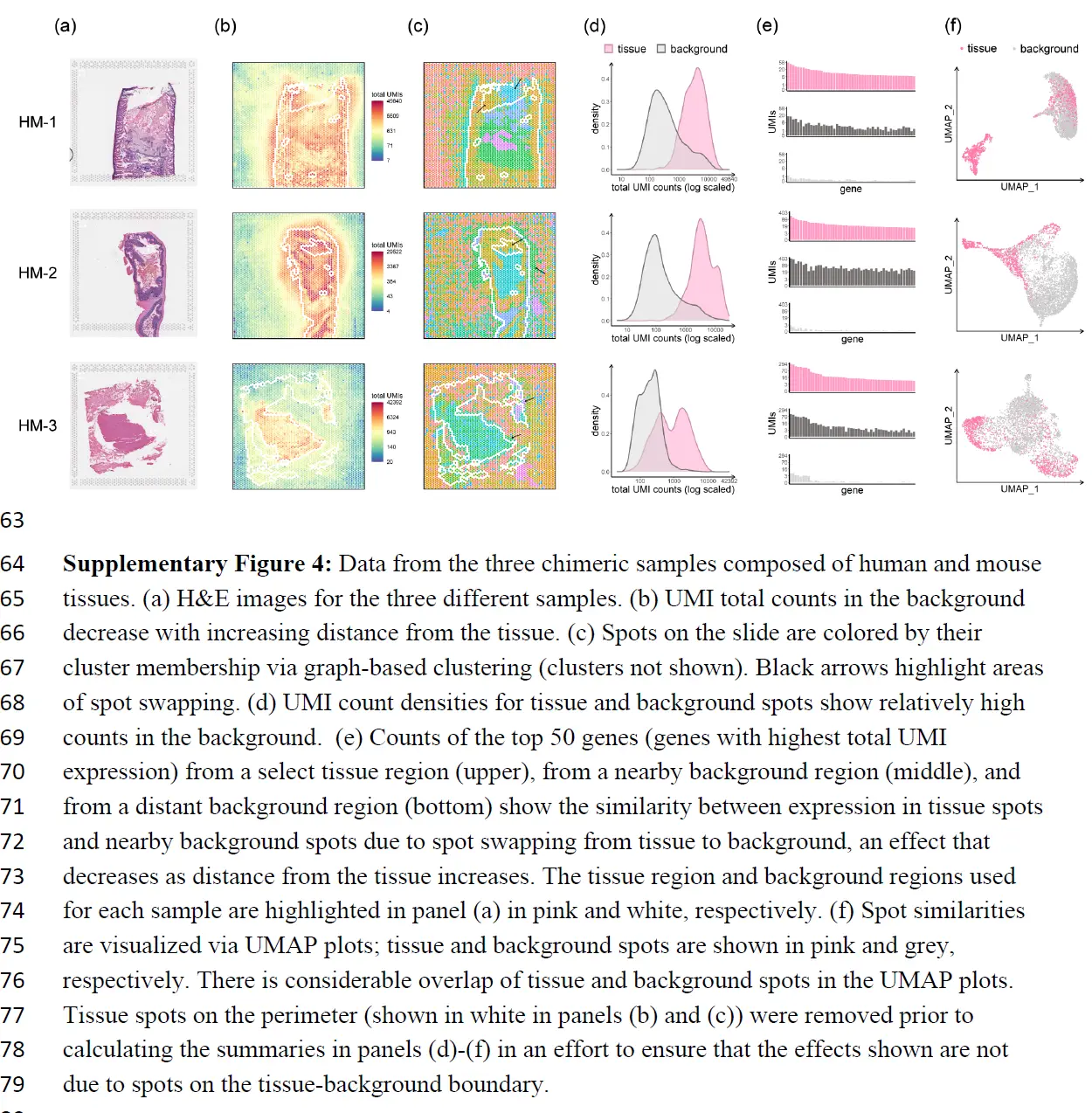
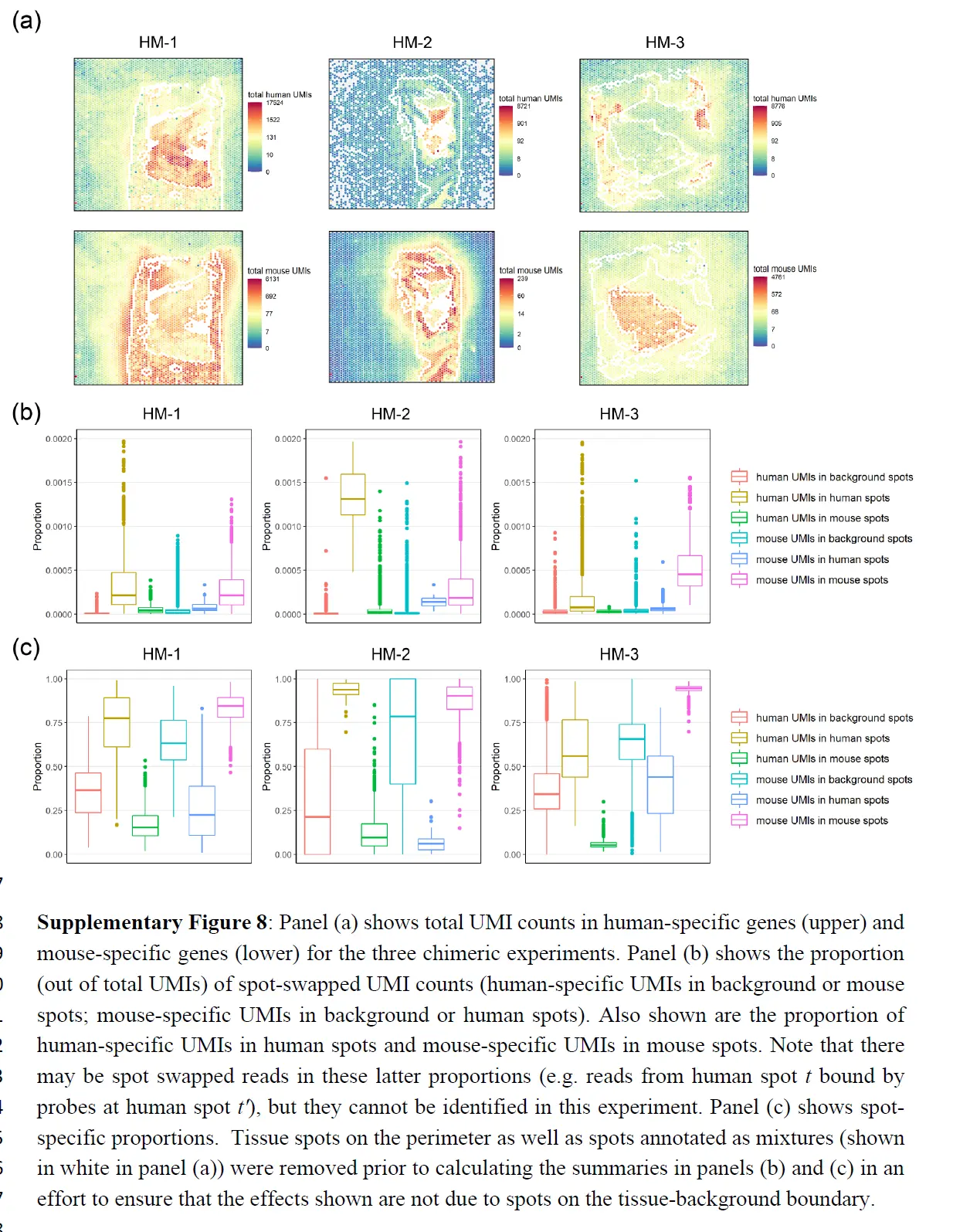
为了更直接地量化点交换的程度,这里进行了嵌合实验,其中人类和小鼠组织在样品制备过程中连续放置。对于每个实验,我们对 H&E 图像进行注释以识别物种特异性区域,并计算点交换读数的比例(人类spot中的小鼠特异性读数、小鼠spot中的人类特异性读数和背景spot中的读数)。这是点交换读数 (LPSS) 比例的下限,因为它不考虑物种内的点交换(例如,来自人类点 t' 处的探针结合的人类点 t 的读数);在这些实验中,LPSS 的范围在 26-37% 之间。总之,组织和背景表达的比较、标记基因分析和嵌合实验(下图)表明点交换影响 ST 实验中的 UMI 计数。
这种令人讨厌的变异性降低了下游分析的能力和精度(下图)。
为调整 RNA-seq 实验中已知污染源而开发的统计方法不适应点交换中固有的空间依赖性,因此,在此设置中是不够的。为了调整 ST 实验中点交换的影响,作者开发了 SpotClean。该方法在 R 包 R/spotClean 中实现。 SpotClean 是根据模拟和案例研究数据进行评估的。在 SimI 中,假设局部污染遵循Gaussian kernel,则生成污染计数; SimII-IV 放宽了高斯假设。在 SimV 中,对平均表达在载玻片上有系统变化的基因的污染计数进行了模拟。下表显示了模拟数据集中真实基因表达和去污染基因表达之间的均方误差 (MSE),
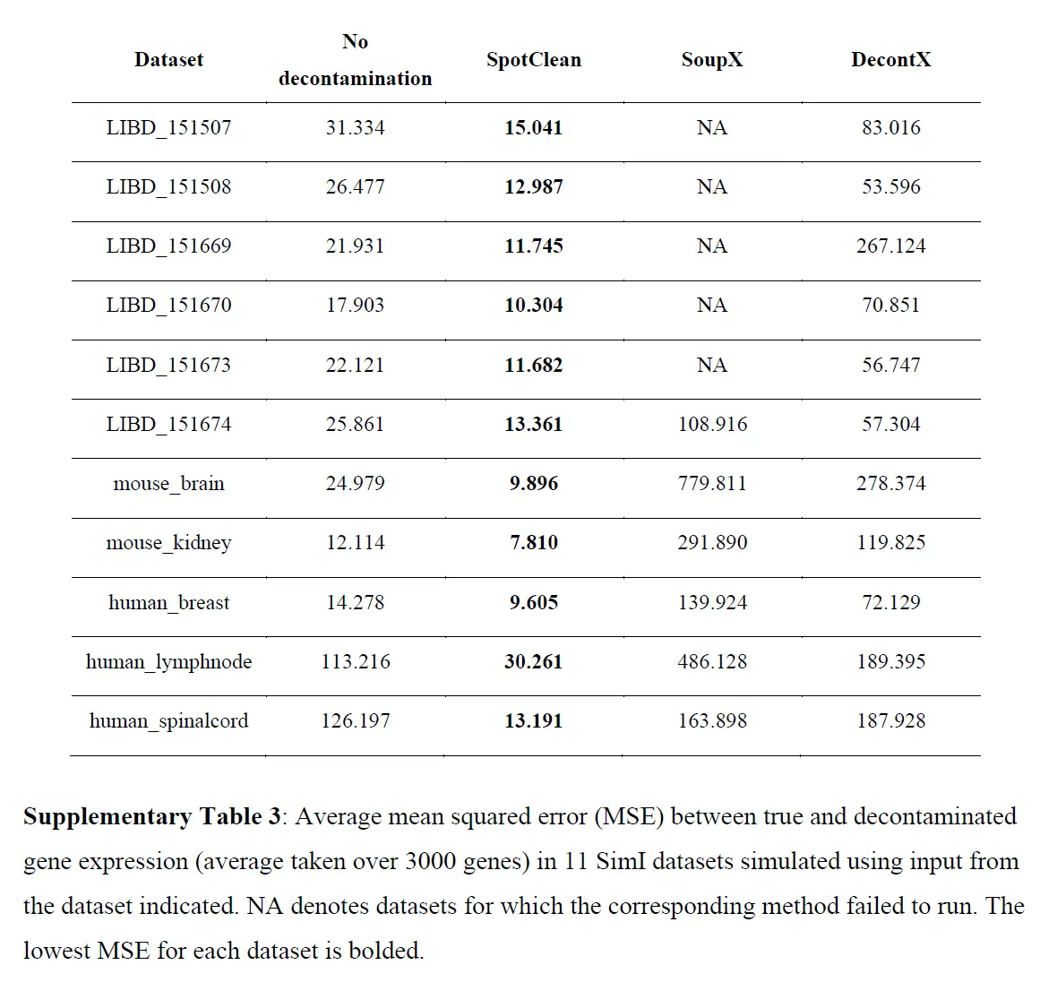
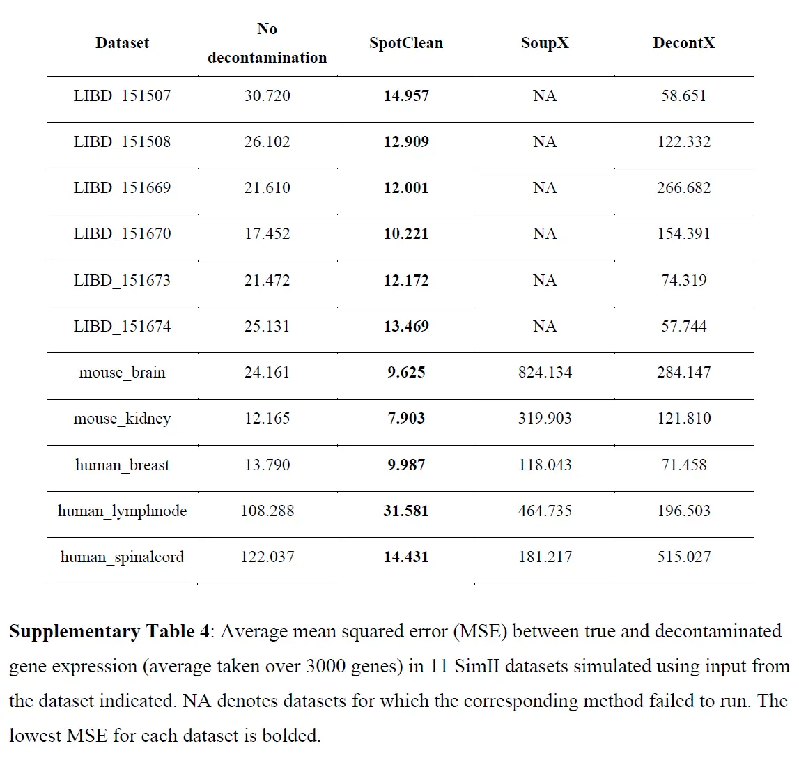
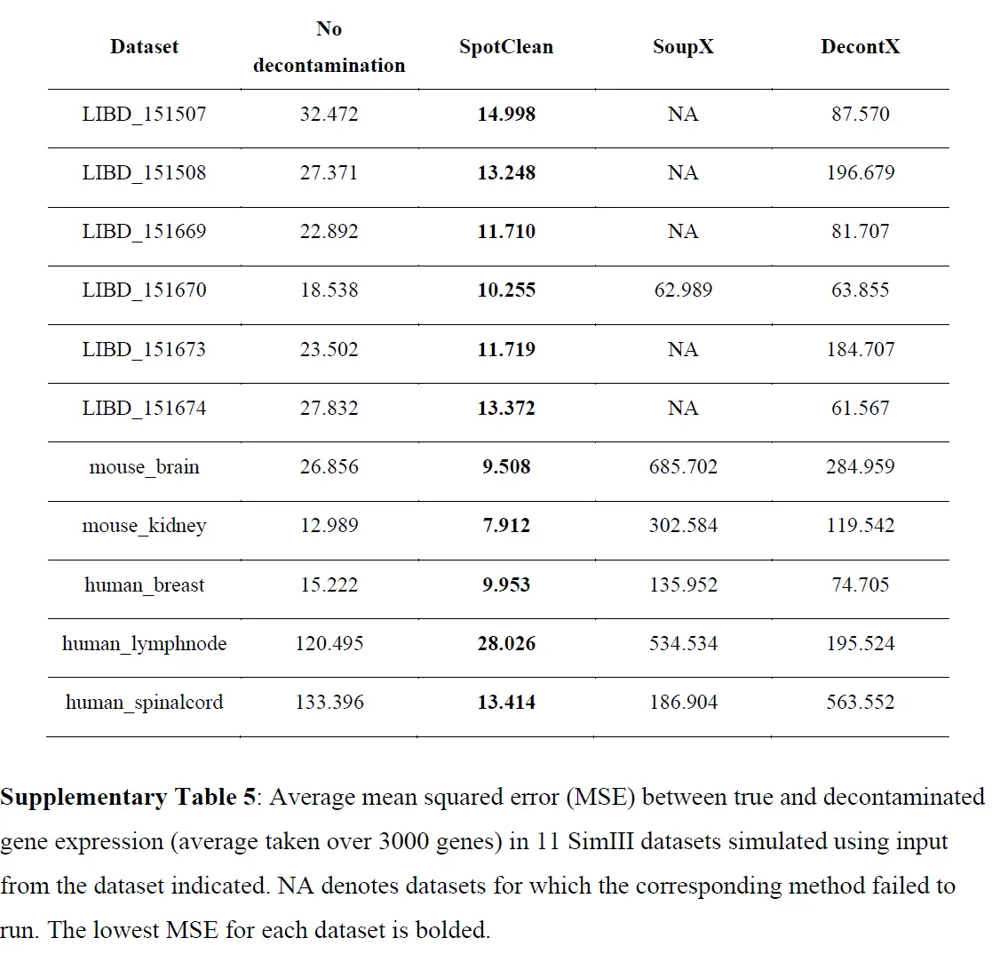
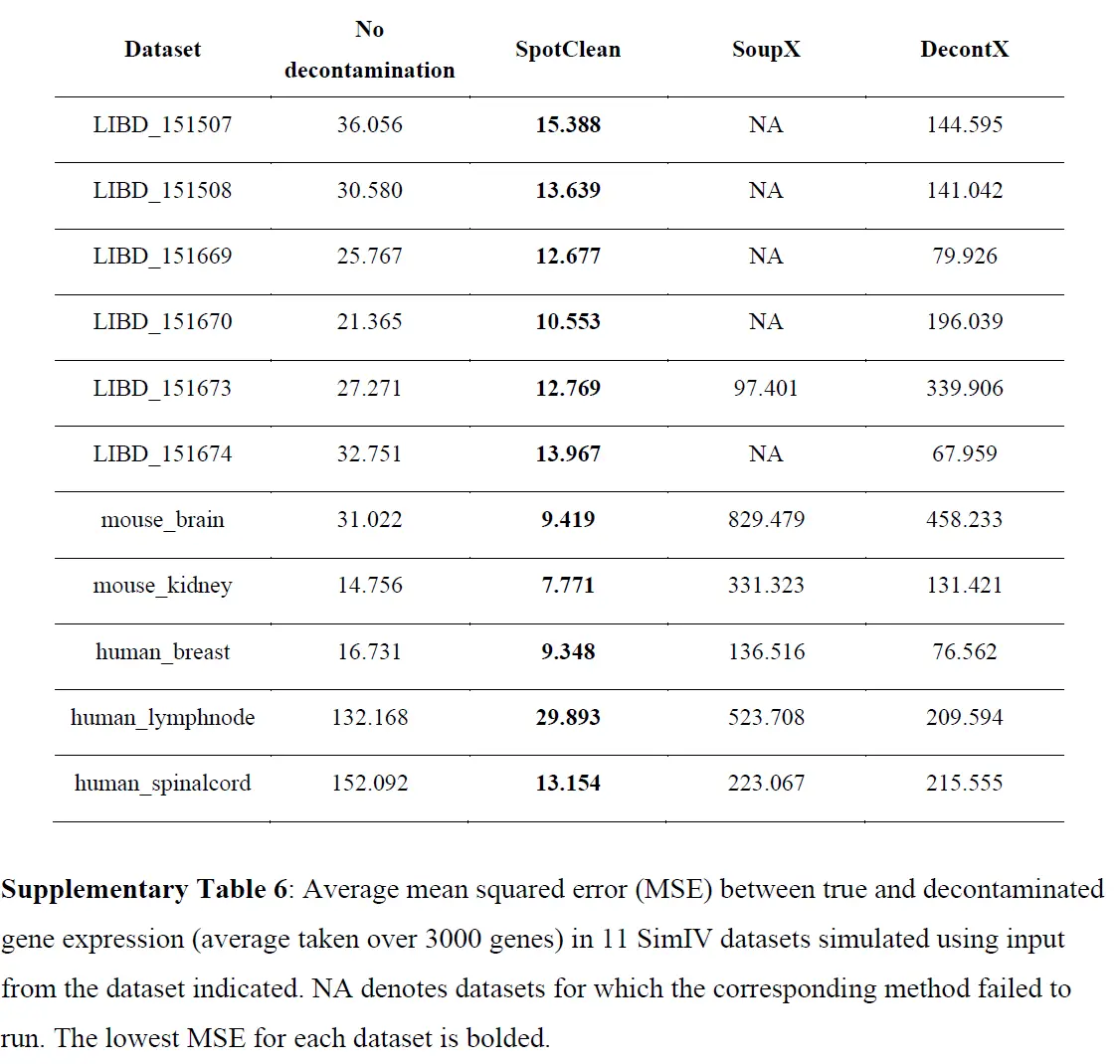
这些结果表明 SpotClean 提供了更好的表达估计;和下图表明,SpotClean 表达估计提高了识别空间变化基因的精度。
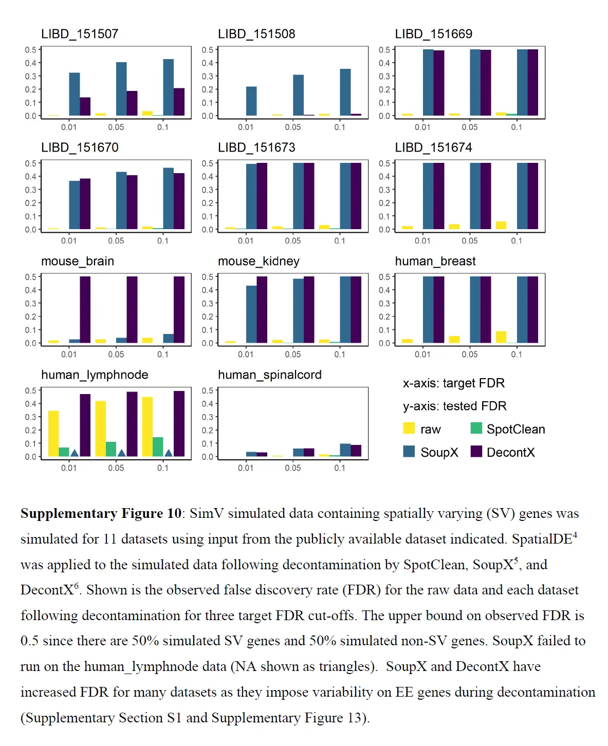
SpotClean 对下游分析的好处也在案例研究数据中得到了说明。 具体来说,SpotClean 增加了标记基因表达的特异性,增加了识别 DE 基因的能力,并提高了斑点注释的准确性。 下图表明SpotClean 通过维持 WM 和 Layer1 中的表达水平并减少其他层中的虚假表达,提高了 SpatialLIBD 数据中 GFAP 的特异性。
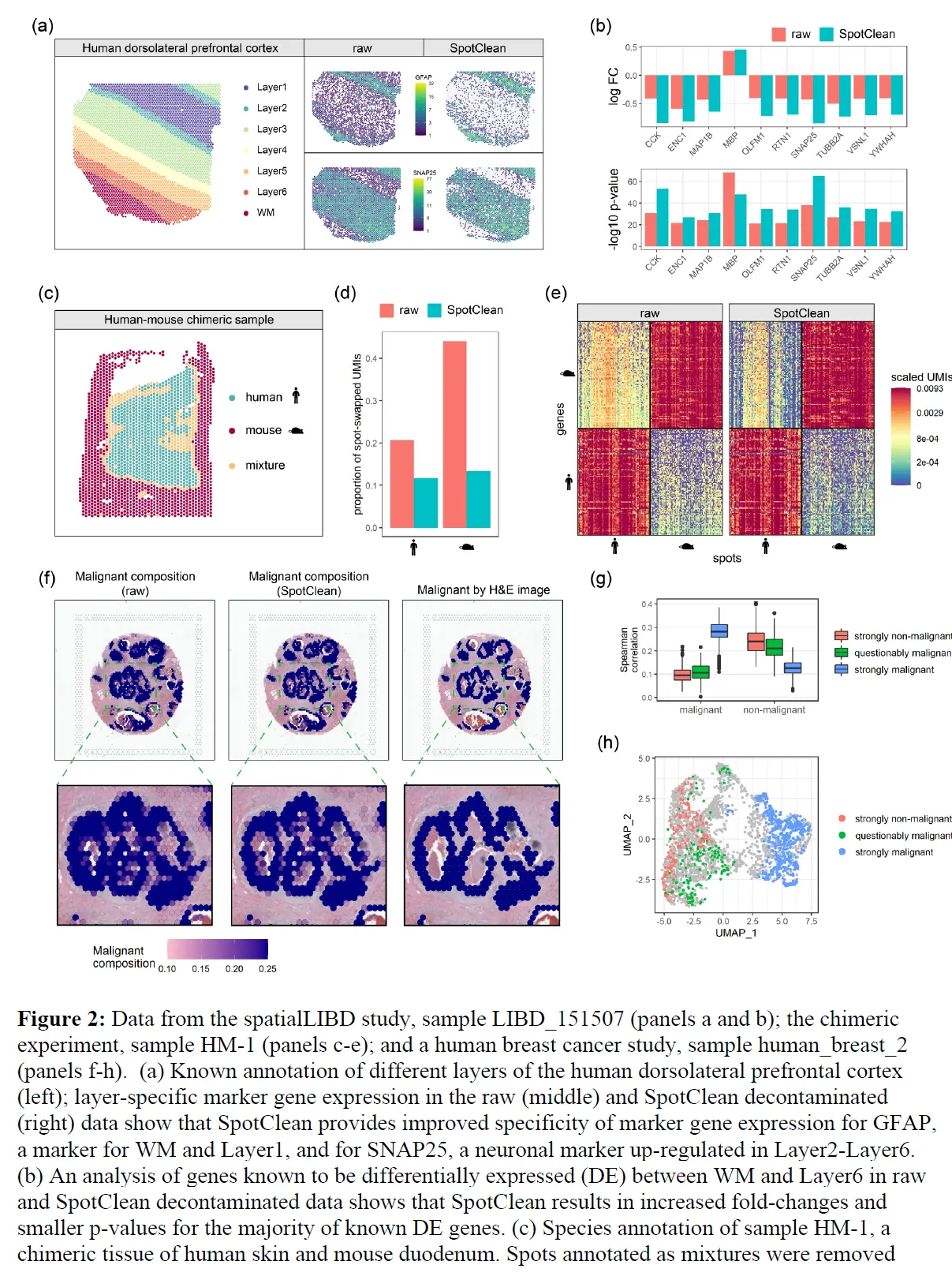
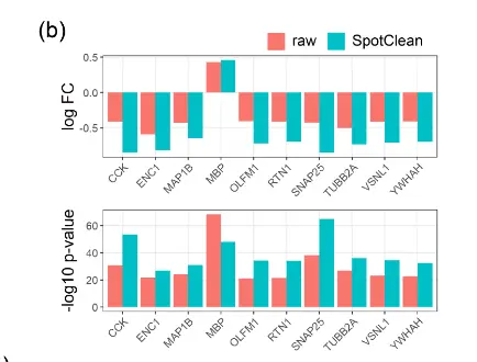
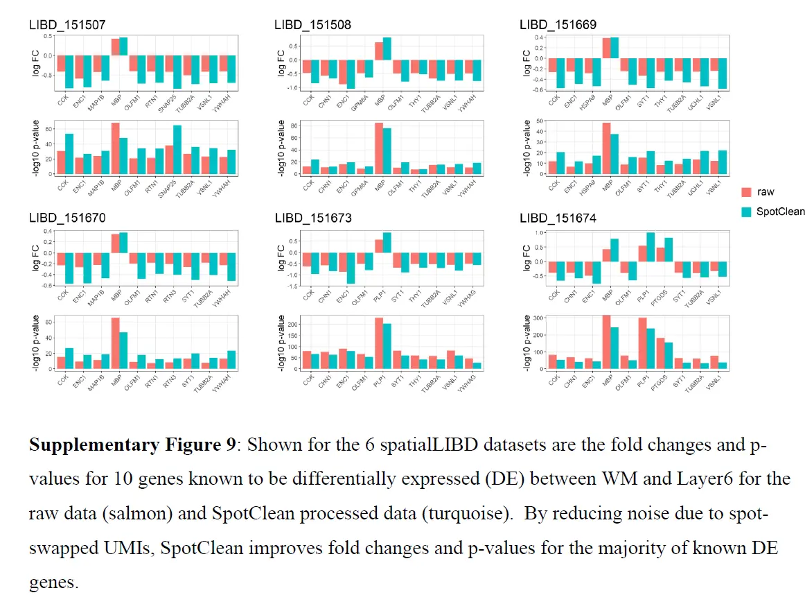
上图b 和下图考虑了已知在原始和 SpotClean 净化数据中 WM 和 Layer6 之间差异表达(DE)的基因;
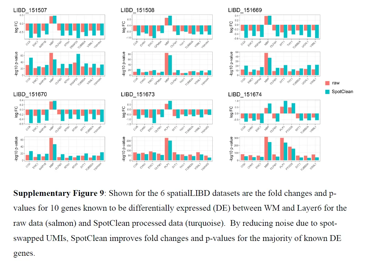
SpotClean 导致已知 DE 基因的倍数变化增加和 p 值减小。 嵌合数据集提供了额外的例子。 特别是,SpotClean 减少了嵌合数据集中点交换 UMI 计数的比例。 类似的结果显示在上图中,考虑到人类特异性和小鼠特异性基因在人类特异性和小鼠特异性位点的表达。 通过 SpotClean 净化的数据显示小鼠组织中人类基因的表达减少,而人体组织没有减少,反之亦然。
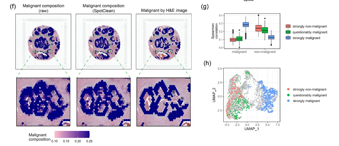
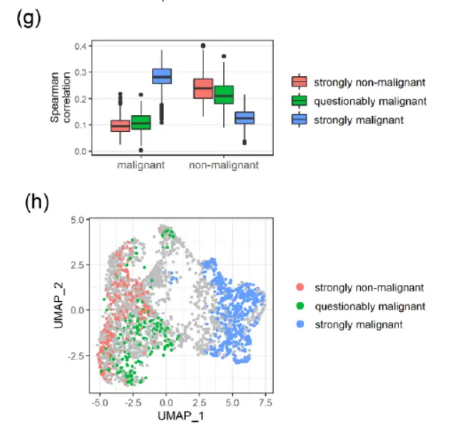
将空间转录组学应用于个性化医疗引起了相当大的兴趣,例如患者肿瘤活检的分子分析以指导诊断和精准治疗。 SpotClean 在精确点注释至关重要的此类应用中展示了巨大的优势。下图显示了人类乳腺癌样本(导管癌),其中肿瘤的诊断、范围和侵袭性通常是通过病理学家对 H&E 图像的评估来估计的。
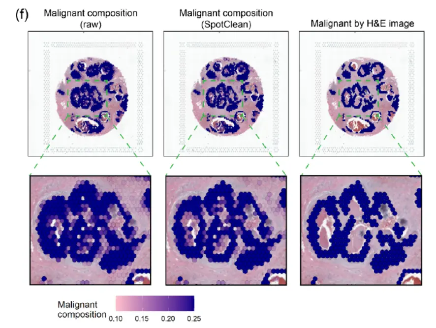
空间转录组学可以提供额外的信息,包括识别恶性细胞的细微集合,但需要准确的spot注释才能使这些信息在临床实践中有用,尤其是不要过度强调肿瘤负荷。上图显示了使用 SpotClean 数据注释的spot与使用未通过 SpotClean 净化的数据注释的spot。未经净化的数据将许多spot误认为是恶性的,包括那些在肿瘤周围含有良性炎症细胞的spot,而 SpotClean 净化的数据更接近于在 H&E 图像上识别恶性细胞。下图显示,在没有 SpotClean 的情况下,原始数据中超过 13% 的标记为恶性的spot可能是由于spot交换造成的误判。
空间转录组学为解决生物学问题和加强患者护理提供了前所未有的机会,但必须调整点交换引起的伪影,以确保从这些强大的实验中获得最大的信息。 SpotClean 提供更准确的表达估计,从而提高下游分析的能力和精度。
最后看看示例代码
安装和加载
if (!requireNamespace("BiocManager", quietly = TRUE))
    install.packages("BiocManager")

BiocManager::install("SpotClean")
library(SpotClean)
Short Demo
在这里,在捆绑的示例数据上快速演示了一般的 SpotClean 工作流程。 然后在下面进行分步说明。
# Not run

# Load example data
data(mbrain_raw)
data(mbrain_slide_info)

# Visualize raw data
mbrain_obj <- CreateSlide(count_mat = mbrain_raw,
                          slide_info = mbrain_slide_info)
VisualizeSlide(slide_obj = mbrain_obj)
VisualizeHeatmap(mbrain_obj,rownames(mbrain_raw)[1])

# Decontaminate raw data
decont_obj <- SpotClean(mbrain_obj)

# Visualize decontaminated gene
VisualizeHeatmap(decont_obj,rownames(mbrain_raw)[1])

# Visualize the estimated per-spot contamination rate
VisualizeHeatmap(decont_obj,decont_obj@metadata$contamination_rate,
                 logged = FALSE, legend_title = "contamination rate",
                 legend_range = c(0,1))

# (Optionally) Transform to Seurat object for downstream analyses
seurat_obj <- ConvertToSeurat(decont_obj,image_dir = "/path/to/spatial/folder")
Running Speed
计算速度与输入数据集的大小和结构有关,主要由组织spot的数量驱动。 SpotClean 不需要并行计算,因此不会占用过多 CPU 或内存资源。 作为参考,SpotClean 在默认基因过滤下在中等大小的数据集(大约 30,000 个基因和 2,000 个组织spot)上运行所需的时间不到 15 分钟。
Situations you should think twice about before applying SpotClean
- $组织斑点过多(背景斑点不够):虽然观察到的数据是具有固定列数(spot)的单个矩阵,但未知参数的数量与组织spot的数量成正比。 在所有spot都被组织覆盖的极端情况下,有比观察到的数据值更多的未知参数。 在这种情况下,受污染的表达式与真实表达式混淆,SpotClean 估计变得不可靠。 因此建议输入数据至少有 25% 的斑点未被组织占据,以便 SpotClean 从背景斑点中获得足够的信息来估计污染。
- Lowly-expressed genes: Lowly-expressed genes typically contain relatively less information and relatively more noise than highly-expressed genes. SpotClean by default only keeps highly-expressed and highly-variable genes for decontamination. It can be forced to run on manually-specified lowly-expressed genes. However, even in this case, expression for the lowly-expressed genes is typically not changed very much. Given the high sparsity in most lowly expressed genes, there is not enough information available to confidently reassign UMIs in most cases. However, we do not filter genes by sparsity because there can be interesting genes highly concentrated in a small tissue region. In cases like this, SpotClean is effective at adjusting for spot swapping in these regions. If the defaults are not appropriate, users can either adjust the expression cutoffs or manually specify genes to decontaminate.
- Inference based on sequencing depth: SpotClean reassigns bled-out UMIs to their tissue spots of origin which changes the estimated sequencing depth of tissue spots after decontamination, since most estimations of sequencing depth rely on total expressions at every spot. As a result, decontamination can be considered as another type of normalization and might conflict with existing sequencing depth normalization methods.
Recommended applications
SpotClean 通过校正点交换来改进表达的估计。 换句话说,SpotClean 通过增强高表达区域的信号并减少未表达区域的测量信号来降低噪声。 因此,SpotClean 将提高基于标记基因的推断的准确性,包括组织类型注释、细胞类型分解、与单细胞 RNA-seq 数据的集成以及相关的下游分析。 SpotClean 还改进了空间可变和差异表达 (DE) 基因的识别。 注意到,在某些情况下,由于spot组内的变异性增加,与已知 DE 基因相关的 p 值可能会在 SpotClean 后略微增加(即真正表达的区域变得更高表达;并且从未表达的区域中去除信号)。
鉴于cluster主要由相对较少的高表达基因决定,SpotClean 不会在大多数数据集中显着改变cluster。 虽然cluster的定义可能会稍微好一些,但在大多数情况下,在应用 SpotClean 后,看不到cluster数量和/或cluster之间关系的差异。
step-to-step analyse
加载10X空间数据
# Not run

raw_mat <- Read10xRaw(count_dir = "/path/to/raw_feature_bc_matrix/")
slide_info <- Read10xSlide(tissue_csv_file="/path/to/tissue_positions_list.csv",
                           tissue_img_file="/path/to/tissue_lowres_image.png",
                           scale_factor_file="/path/to/scalefactors_json.json")

# Compare with bundled example data
data(mbrain_raw)
data(mbrain_slide_info)
slide_info$slide$total_counts <- colSums(
    raw_mat[rownames(mbrain_raw),mbrain_slide_info$slide$barcode]
)

identical(raw_mat[rownames(mbrain_raw),], mbrain_raw)
identical(slide_info$slide, mbrain_slide_info$slide)
Create the slide object
data(mbrain_raw)
data(mbrain_slide_info)

slide_obj <- CreateSlide(mbrain_raw, mbrain_slide_info)
slide_obj
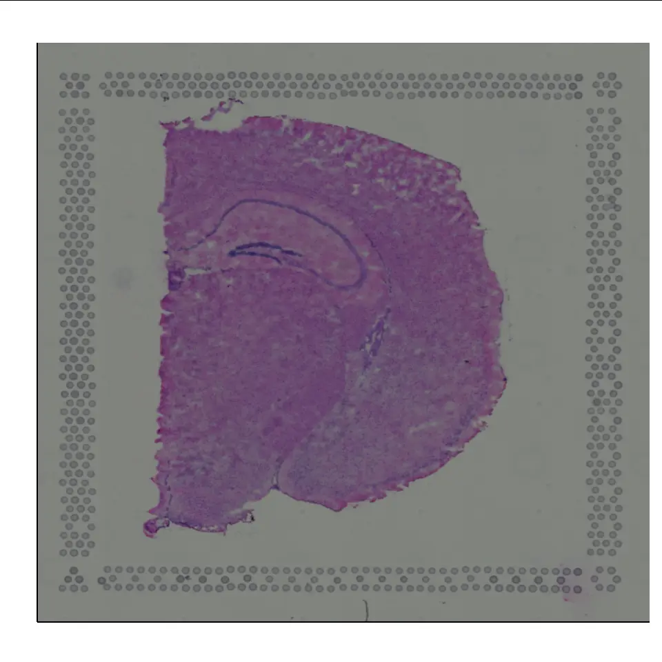
Visualize the slide object
VisualizeSlide(slide_obj)
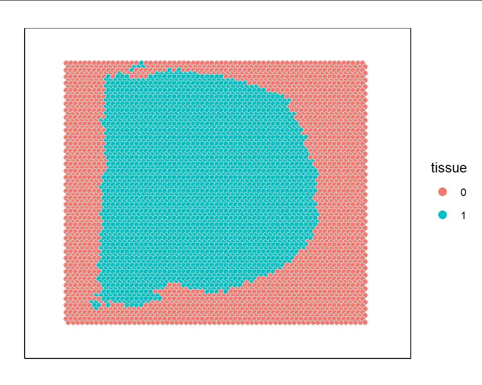
Function VisualizeLabel() shows the spot labels. You can specify the column name of character labels in the slide metadata, or manually provide a vector of character labels corresponding to each spot. For example, we can plot their tissue/background labels, which has been pre-stored in the input slide information:
VisualizeLabel(slide_obj,"tissue")
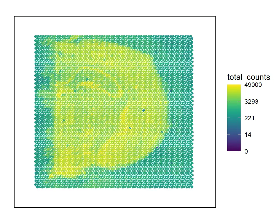
Function VisualizeHeatmap() draws a heatmap of values at every spot in the 2-D slide space. Similar to VisualizeLabel(), you can specify the column name of numerical values in the slide metadata, or manually provide a vector of numerical values corresponding to each spot. For example, we can plot the total UMI counts in every spot, which again has been pre-stored in the input slide information:
VisualizeHeatmap(slide_obj,"total_counts")
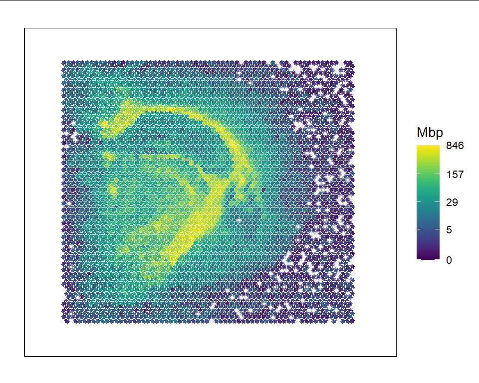
You can also provide a certain gene name appearing in the raw count matrix in input slide object to VisualizeHeatmap(). For example, the expression of the Mbp gene can be visualized:
VisualizeHeatmap(slide_obj,"Mbp")
VisualizeLabel() and VisualizeHeatmap() both support manual label/value inputs, subsetting spots to plot, title and legend name modification. VisualizeHeatmap() also supports different color palettes (rainbow vs. viridis) and log-scaling options. These visualization functions return ggplot2 objects, which can be further modified by users.
Decontaminate the data
SpotClean() is the main function for performing decontamination. It takes the slide object of raw data as input together with some parameters for controlling optimization and convergence, and returns a slide object with decontaminated gene expressions and other model-related parameters and statistics appending to the slide information. Detailed parameter explanations can be found by running ?SpotClean. Here we set maxit=10 and candidate_radius=20 to save computation time. In practice, SpotClean() by default evaluates a series of candidate radii and automatically chooses the best one. The default maximum number of iterations is 30, which can be extended if convergence has not been reached.
decont_obj <- SpotClean(slide_obj, maxit=10, candidate_radius = 20)
meta数据现在包含更多信息,包括来自 SpotClean 模型的参数估计和污染水平的测量。
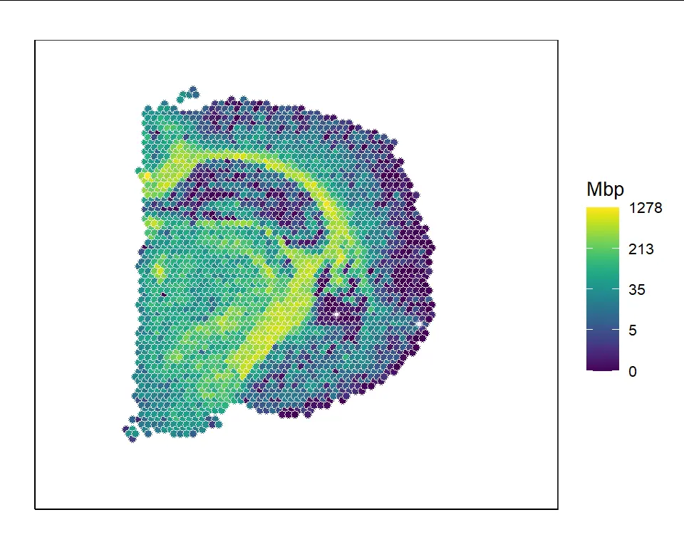
We can visualize the Mbp gene expressions after 10 iterations of decontamination:
VisualizeHeatmap(decont_obj,"Mbp")
Estimate contamination levels in observed data
Our model is able to estimate the proportion of contaminated expression at each tissue spot (i.e. expression at a tissue spot that orginated from a different spot due to spot swapping):
summary(decont_obj@metadata$contamination_rate)
This indicates around 30% of UMIs at a tissue spot in the observed data came from spot swapping contamination, averaging across all tissue spots.
ARC score
还提供了另一种污染水平的主观估计,称为环境 RNA 污染 (ARC) 分数。 它可以使用函数 ARCScore() 计算,也是去污输出的一部分。 直观地,ARC 分数是观察到的组织斑点中污染比例的保守下限。 ARC 分数还可以应用于基于液滴的单细胞数据,以在用空液滴替换背景点时估计环境 RNA 污染。 可以通过运行 ?ARCScore 找到详细信息。
ARCScore(slide_obj)
## [1] 0.05160659
This indicates at least 5% expressions in observed data came from spot swapping contamination.
Convert to Seurat object for downstream analyses
ConvertToSeurat() can be used to convert our slide object to a Seurat spatial object. Note that Seurat requires full input of the spatial folder. In the above example, this is the spatial folder.
seurat_obj <- ConvertToSeurat(decont_obj,image_dir = "/path/to/spatial/folder")
生活很好,有你更好


 1773
1773

 被折叠的 条评论
为什么被折叠?
被折叠的 条评论
为什么被折叠?
 到【灌水乐园】发言


