【模型学习】CLIP_对比语言-图像预训练

参考：http://t.csdnimg.cn/ufifE

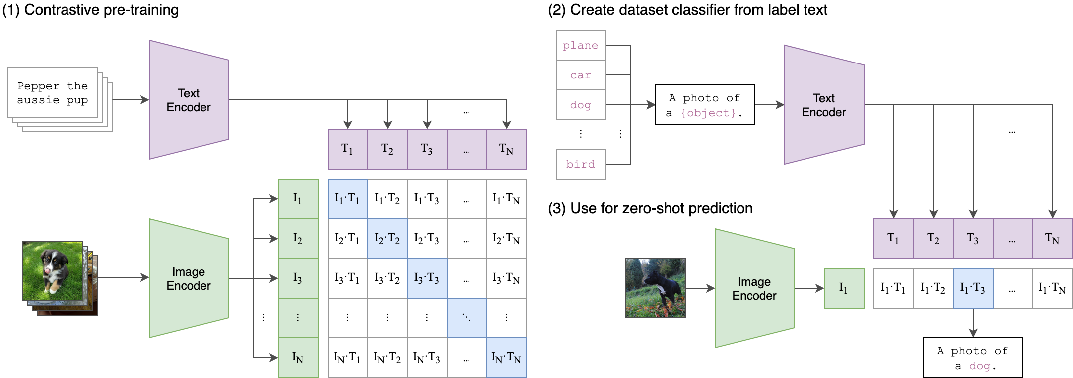
CLIP的全称是Contrastive Language-Image Pre-Training，中文是对比语言-图像预训练。

CLIP的主要目标是通过对比学习，学习匹配图像和文本。在训练过程中，模型学会了将图像和文本编码成统一的向量空间，这使得它能够在语言和视觉上理解它们之间的关系。通过这种方式，CLIP可以识别图像中的物体、场景、动作等元素，同时也能够理解与图像相关的文本，例如标签、描述、标题等。

CLIP的基本原理是对比学习，即让模型学习区分正样本（匹配的图像和文本对）和负样本（不匹配的图像和文本对）。为了实现这一目标，CLIP使用了一个多模态编码器，它由两个子编码器组成：一个用于图像，一个用于文本。图像编码器可以是基于卷积神经网络（CNN）或者视觉变换器（ViT）的模型，文本编码器则是一个基于Transformer的模型。这两个编码器都可以将输入转换为一个固定长度的向量表示，然后通过计算向量之间的余弦相似度来衡量图像和文本之间的匹配程度。

CLIP模型在各种图像分类任务上表现优异，包括对一般图像、细粒度分类、检索任务和少样本学习的支持。同时，它还能够识别和理解图像中的复杂概念，比如人类行为、建筑物和文化符号等，这对于各种视觉应用非常有用。

CLIP的应用非常广泛，包括图像检索、视觉问答、视觉导航、图像生成等等。此外，OpenAI还推出了一个名为DALL-E的模型，它是在CLIP模型的基础上开发的一种生成模型，能够基于自然语言描述生成图像。

模型架构

使用示例：

import torch
import clip
from PIL import Image

# 加载预训练模型
model, preprocess = clip.load('ViT-B/32', device='cpu')

# 加载图像
image = Image.open('image.jpg')

# 对图像进行预处理
image_input = preprocess(image).unsqueeze(0)

# 运行模型
with torch.no_grad():
    image_features = model.encode_image(image_input)

# 加载类别标签
class_labels = ['cat', 'dog', 'flower', 'food', 'car']

# 加载类别描述
class_descriptions = clip.tokenize(class_labels).to(model.device)

# 计算图像与类别描述之间的相似度
logits_per_image, logits_per_text = model(image_input, class_descriptions)
probas = logits_per_image.softmax(dim=-1).cpu().numpy()

# 输出预测结果
for i, class_label in enumerate(class_labels):
    print(f"{class_label}: {probas[0][i]}")

---

网络结构 

Image encoder

第一部分

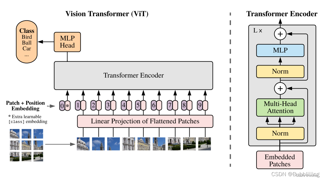
先卷积，卷积后添加class token，获得序列信息

class VisionTransformer(nn.Module):
    def __init__(self, input_resolution: int, patch_size: int, width: int, layers: int, heads: int, output_dim: int):
        super().__init__()
        self.input_resolution = input_resolution
        self.output_dim = output_dim
        #-----------------------------------------------#
        #   224, 224, 3 -> 196, 768
        #-----------------------------------------------#
        self.conv1 = nn.Conv2d(in_channels=3, out_channels=width, kernel_size=patch_size, stride=patch_size, bias=False)

        scale = width ** -0.5
        #--------------------------------------------------------------------------------------------------------------------#
        #   class_embedding部分是transformer的分类特征。用于堆叠到序列化后的图片特征中，作为一个单位的序列特征进行特征提取。
        #
        #   在利用步长为16x16的卷积将输入图片划分成14x14的部分后，将14x14部分的特征平铺，一幅图片会存在序列长度为196的特征。
        #   此时生成一个class_embedding，将class_embedding堆叠到序列长度为196的特征上，获得一个序列长度为197的特征。
        #   在特征提取的过程中，class_embedding会与图片特征进行特征的交互。最终分类时，我们取出class_embedding的特征，利用全连接分类。
        #--------------------------------------------------------------------------------------------------------------------#
        #   196, 768 -> 197, 768
        self.class_embedding = nn.Parameter(scale * torch.randn(width))
        #--------------------------------------------------------------------------------------------------------------------#
        #   为网络提取到的特征添加上位置信息。
        #   以输入图片为224, 224, 3为例，我们获得的序列化后的图片特征为196, 768。加上class_embedding后就是197, 768
        #   此时生成的pos_Embedding的shape也为197, 768，代表每一个特征的位置信息。
        #--------------------------------------------------------------------------------------------------------------------#
        #   197, 768 -> 197, 768
        self.positional_embedding = nn.Parameter(scale * torch.randn((input_resolution // patch_size) ** 2 + 1, width))

    def forward(self, x: torch.Tensor):
        x = self.conv1(x)  # shape = [*, width, grid, grid]
        x = x.reshape(x.shape[0], x.shape[1], -1)  # shape = [*, width, grid ** 2]
        x = x.permute(0, 2, 1)  # shape = [*, grid ** 2, width]
        x = torch.cat([self.class_embedding.to(x.dtype) + torch.zeros(x.shape[0], 1, x.shape[-1], dtype=x.dtype, device=x.device), x], dim=1)  # shape = [*, grid ** 2 + 1, width]
        x = x + self.positional_embedding.to(x.dtype)

序列信息放入Transformer encoder进行特征提取（Transformer特有的Multi-head Self-attention结构）

---

自注意力

self-attention常规计算

如果我们想要获得input-1的输出，那么我们进行如下几步： 1、利用input-1的查询向量，分别乘上input-1、input-2、input-3的键向量，此时我们获得了三个score。 2、然后对这三个score取softmax，获得了input-1、input-2、input-3各自的重要程度。 3、然后将这个重要程度乘上input-1、input-2、input-3的值向量，求和。 4、此时我们获得了input-1的输出。

如图所示，我们进行如下几步： 1、input-1的查询向量为[1, 0, 2]，分别乘上input-1、input-2、input-3的键向量，获得三个score为2，4，4。 2、然后对这三个score取softmax，获得了input-1、input-2、input-3各自的重要程度，获得三个重要程度为0.0，0.5，0.5。 3、然后将这个重要程度乘上input-1、input-2、input-3的值向量，求和，即 0.0 ∗ [ 1 , 2 , 3 ] + 0.5 ∗ [ 2 , 8 , 0 ] + 0.5 ∗ [ 2 , 6 , 3 ] = [ 2.0 , 7.0 , 1.5 ] 0.0 * [1, 2, 3] + 0.5 * [2, 8, 0] + 0.5 * [2, 6, 3] = [2.0, 7.0, 1.5]0.0∗[1,2,3]+0.5∗[2,8,0]+0.5∗[2,6,3]=[2.0,7.0,1.5]。 4、此时我们获得了input-1的输出 [2.0, 7.0, 1.5]。

self-attention的矩阵运算

例：
 

首先利用 查询向量query 叉乘 转置后的键向量key，这一步可以通俗的理解为，利用查询向量去查询序列的特征，获得序列每个部分的重要程度score。 

然后利用 score 叉乘 value，这一步可以通俗的理解为，将序列每个部分的重要程度重新施加到序列的值上去。 

import numpy as np

def soft_max(z):
    t = np.exp(z)
    a = np.exp(z) / np.expand_dims(np.sum(t, axis=1), 1)
    return a

Query = np.array([
    [1,0,2],
    [2,2,2],
    [2,1,3]
])

Key = np.array([
    [0,1,1],
    [4,4,0],
    [2,3,1]
])

Value = np.array([
    [1,2,3],
    [2,8,0],
    [2,6,3]
])

scores = Query @ Key.T
print(scores)
scores = soft_max(scores)
print(scores)
out = scores @ Value
print(out)

---

第二部分 

在完成MultiHeadSelfAttention的构建后，我们需要在其后加上两个全连接。就构建了整个TransformerBlock。

整个VIT模型由一个Patch+Position Embedding加上多个TransformerBlock组成。典型的TransforerBlock的数量为12个。

from collections import OrderedDict

import torch
from torch import nn


class LayerNorm(nn.LayerNorm):
    """Subclass torch's LayerNorm to handle fp16."""

    def forward(self, x: torch.Tensor):
        orig_type = x.dtype
        ret = super().forward(x.type(torch.float32))
        return ret.type(orig_type)


class QuickGELU(nn.Module):
    def forward(self, x: torch.Tensor):
        return x * torch.sigmoid(1.702 * x)


class ResidualAttentionBlock(nn.Module):
    def __init__(self, d_model: int, n_head: int, attn_mask: torch.Tensor = None):
        super().__init__()

        self.attn = nn.MultiheadAttention(d_model, n_head)
        self.ln_1 = LayerNorm(d_model)
        self.mlp = nn.Sequential(OrderedDict([
            ("c_fc", nn.Linear(d_model, d_model * 4)),
            ("gelu", QuickGELU()),
            ("c_proj", nn.Linear(d_model * 4, d_model))
        ]))
        self.ln_2 = LayerNorm(d_model)
        self.attn_mask = attn_mask

    def attention(self, x: torch.Tensor):
        self.attn_mask = self.attn_mask.to(dtype=x.dtype, device=x.device) if self.attn_mask is not None else None
        return self.attn(x, x, x, need_weights=False, attn_mask=self.attn_mask)[0]

    def forward(self, x: torch.Tensor):
        x = x + self.attention(self.ln_1(x))
        x = x + self.mlp(self.ln_2(x))
        return x


class Transformer(nn.Module):
    def __init__(self, width: int, layers: int, heads: int, attn_mask: torch.Tensor = None):
        super().__init__()
        self.width = width
        self.layers = layers
        self.resblocks = nn.Sequential(*[ResidualAttentionBlock(width, heads, attn_mask) for _ in range(layers)])

    def forward(self, x: torch.Tensor):
        return self.resblocks(x)


class VisionTransformer(nn.Module):
    def __init__(self, input_resolution: int, patch_size: int, width: int, layers: int, heads: int, output_dim: int):
        super().__init__()
        self.input_resolution = input_resolution
        self.output_dim = output_dim
        #-----------------------------------------------#
        #   224, 224, 3 -> 196, 768
        #-----------------------------------------------#
        self.conv1 = nn.Conv2d(in_channels=3, out_channels=width, kernel_size=patch_size, stride=patch_size, bias=False)

        scale = width ** -0.5
        #--------------------------------------------------------------------------------------------------------------------#
        #   class_embedding部分是transformer的分类特征。用于堆叠到序列化后的图片特征中，作为一个单位的序列特征进行特征提取。
        #
        #   在利用步长为16x16的卷积将输入图片划分成14x14的部分后，将14x14部分的特征平铺，一幅图片会存在序列长度为196的特征。
        #   此时生成一个class_embedding，将class_embedding堆叠到序列长度为196的特征上，获得一个序列长度为197的特征。
        #   在特征提取的过程中，class_embedding会与图片特征进行特征的交互。最终分类时，我们取出class_embedding的特征，利用全连接分类。
        #--------------------------------------------------------------------------------------------------------------------#
        #   196, 768 -> 197, 768
        self.class_embedding = nn.Parameter(scale * torch.randn(width))
        #--------------------------------------------------------------------------------------------------------------------#
        #   为网络提取到的特征添加上位置信息。
        #   以输入图片为224, 224, 3为例，我们获得的序列化后的图片特征为196, 768。加上class_embedding后就是197, 768
        #   此时生成的pos_Embedding的shape也为197, 768，代表每一个特征的位置信息。
        #--------------------------------------------------------------------------------------------------------------------#
        #   197, 768 -> 197, 768
        self.positional_embedding = nn.Parameter(scale * torch.randn((input_resolution // patch_size) ** 2 + 1, width))
        self.ln_pre = LayerNorm(width)

        self.transformer = Transformer(width, layers, heads)

        self.ln_post = LayerNorm(width)
        self.proj = nn.Parameter(scale * torch.randn(width, output_dim))

    def forward(self, x: torch.Tensor):
        x = self.conv1(x)  # shape = [*, width, grid, grid]
        x = x.reshape(x.shape[0], x.shape[1], -1)  # shape = [*, width, grid ** 2]
        x = x.permute(0, 2, 1)  # shape = [*, grid ** 2, width]
        x = torch.cat([self.class_embedding.to(x.dtype) + torch.zeros(x.shape[0], 1, x.shape[-1], dtype=x.dtype, device=x.device), x], dim=1)  # shape = [*, grid ** 2 + 1, width]
        x = x + self.positional_embedding.to(x.dtype)
        x = self.ln_pre(x)

        x = x.permute(1, 0, 2)  # NLD -> LND
        x = self.transformer(x)
        x = x.permute(1, 0, 2)  # LND -> NLD

        x = self.ln_post(x[:, 0, :])

        if self.proj is not None:
            x = x @ self.proj

        return x

---

Text encoder

Text Encoder是一个基本的Bert，在CLIP中，Text Encoder由12层的Transformer Encoder组成。（由于文本信息相比于视觉信息更加简单，因此每一个规模的CLIP使用到的Text Encoder没有变化，大小都是一样的。）

在CLIP中，Text Encoder的宽度（embeddingsize）为512，numhead值为512/64=8，层数为12，Transformer Encoder，如上图所hi由Self-Attention模块+FFN（Feed Foward Network，本质上就是俩全连接组成），结构非常简单。

在Text Encoder中，我们会对每个句子增加一个Class Token，用于整合特征，以一个固定长度向量来代表输入句子。一般的Bert会将Class Token放在第0位，也就是最前面。而在CLIP中，Class Token被放在了文本的最后。

from collections import OrderedDict

import numpy as np
import torch
import torch.nn as nn
import torch.nn.functional as F

#--------------------------------------#
#   Gelu激活函数的实现
#   利用近似的数学公式
#--------------------------------------#
class GELU(nn.Module):
    def __init__(self):
        super(GELU, self).__init__()

    def forward(self, x):
        return 0.5 * x * (1 + F.tanh(np.sqrt(2 / np.pi) * (x + 0.044715 * torch.pow(x,3))))
    
class ResidualAttentionBlock(nn.Module):
    def __init__(self, d_model: int, n_head: int, attn_mask: torch.Tensor = None):
        super().__init__()

        self.attn = nn.MultiheadAttention(d_model, n_head)
        self.ln_1 = nn.LayerNorm(d_model)
        self.mlp = nn.Sequential(OrderedDict([
            ("c_fc", nn.Linear(d_model, d_model * 4)),
            ("gelu", GELU()),
            ("c_proj", nn.Linear(d_model * 4, d_model))
        ]))
        self.ln_2 = nn.LayerNorm(d_model)
        self.attn_mask = attn_mask

    def attention(self, x: torch.Tensor):
        self.attn_mask = self.attn_mask.to(dtype=x.dtype, device=x.device) if self.attn_mask is not None else None
        return self.attn(x, x, x, need_weights=False, attn_mask=self.attn_mask)[0]

    def forward(self, x: torch.Tensor):
        x = x + self.attention(self.ln_1(x))
        x = x + self.mlp(self.ln_2(x))
        return x

class Transformer(nn.Module):
    def __init__(self, width: int, layers: int, heads: int, attn_mask: torch.Tensor = None):
        super().__init__()
        self.width = width
        self.layers = layers
        self.resblocks = nn.Sequential(*[ResidualAttentionBlock(width, heads, attn_mask) for _ in range(layers)])

    def forward(self, x: torch.Tensor):
        return self.resblocks(x)

---

模型训练

假设一个批次中有64个文本图像对，此时我们会同时获得64个图片和64个文本，首先我们从64个文本图像对中取出一个文本图像对，成对的文本图像对是天然的正样本，它们是配对的。

而对于这个样本的文本来讲，其它63个图像都为负样本，它们是不配对的。 而对于这个样本的图像来讲，其它63个文本都为负样本，它们是不配对的。

我们使用visualembedding 叉乘 textembedding，得到一个[64, 64]的矩阵，那么对角线上的值便是成对特征内积得到的，如果visualembedding和对应的textembedding越相似，那么它的值便越大。

我们选取[64, 64]矩阵中的第一行，代表第1个图片与64个文本的相似程度，其中第1个文本是正样本，我们将这一行的标签设置为1，那么我们就可以使用交叉熵进行训练，尽量把第1个图片和第一个文本的内积变得更大，那么它们就越相似。

---

代码下载 

openai_github仓库