生信游民作业—两次差异分析结果交集需要有多大才算是一致呢(第二部分)

学徒作业

​ 理论上，任意疾病或者其它实验设计，都是可以找到多个数据集，它们各自可以独立差异分析。然后，使用下面的统计学方法和工具来进行比较：1.Jaccard相似性指数；2.Pearson相关系数；3. Spearman秩相关系数；4. Venn图；5. Gene Set Enrichment分析(GSEA); 6. 差异基因列表重叠分析; 7. 回归分析。

​ 上一部分我展示了芯片数据差异分析的基础流程，在这一部分我将对获得的两组差异基因使用统计学方法和工具进行比较。

一、分别对两个数据集的上下调基因进行富集分析:

​ 这一部分是初步看一下上下调基因分别富集在哪些通路中，两组数据是否相似。

1.输入数据及加载R包

rm(list = ls())
library(clusterProfiler)
library(ggthemes)
library(org.Hs.eg.db)
library(dplyr)
library(ggplot2)
library(stringr)
library(enrichplot)
library(forcats)
GSE9844 <- read.csv("GSE9844-degs.csv", header = T, check.names = T)
GSE13601 <- read.csv("GSE13601-degs.csv", header = T, check.names = T)
# 上述的degs就是上一部分获得的差异基因

2.提取差异基因

Degs_GSE9844 <- GSE9844[!GSE9844$change == "stable",]
Degs_GSE13601 <- GSE13601[!GSE13601$change == "stable",]

up_GSE9844 <- GSE9844[GSE9844$change == "up",]
down_GSE9844 <- GSE9844[GSE9844$change == "down",]

up_GSE13601 <- GSE13601[GSE13601$change == "up",]
down_GSE13601 <- GSE13601[GSE13601$change == "down",]

3.UP基因模块(仅展示一组数据的处理过程)

#KEGG、GO富集
kegg_up_results <- enrichKEGG(gene  = up_GSE9844$ENTREZID,
                              organism  = "hsa", #物种人类 hsa 小鼠mmu
                              pvalueCutoff = 0.05, #默认0.05
                              qvalueCutoff = 0.2, #默认0.2
                              minGSSize = 0,  #默认是10
                              maxGSSize = 500 #默认是500
)
                            
kegg_up_results <- setReadable(kegg_up_results, 
                               OrgDb="org.Hs.eg.db", 
                               keyType='ENTREZID' #ENTREZID to gene Symbol
)

write.csv(kegg_up_results@result,'KEGG_up_enrichresults.csv') 
save(kegg_up_results, file ='KEGG_up_enrichresults.Rdata')

go_up_enrich_results <- enrichGO(gene = up_GSE9844$ENTREZID,
                                 OrgDb = "org.Hs.eg.db",
                                 ont   = "ALL"  ,     #One of "BP", "MF"  "CC"  "ALL" 
                                 pvalueCutoff = 0.05, #默认0.05
                                 qvalueCutoff = 0.2, #默认0.2
                                 minGSSize = 0,  #默认是10
                                 maxGSSize = 500, #默认是500
                                 readable = TRUE
)

write.csv(go_up_enrich_results@result, 'Go_up_enrichresults.csv') 
save(go_up_enrich_results, file ='Go_up_enrichresults.Rdata')

#setReadable和readable = TRUE都是把富集结果表格里的基因名称转为symbol

4.down基因模块

#KEGG、GO富集
kegg_down_results <- enrichKEGG(gene  = down_GSE9844$ENTREZID,
                                organism  = "hsa", #物种人类 hsa 小鼠mmu
                                pvalueCutoff = 0.05, #默认0.05
                                qvalueCutoff = 0.2, #默认0.2
                                minGSSize = 0,  #默认是10
                                maxGSSize = 500 #默认是500
)

kegg_down_results <- setReadable(kegg_down_results, 
                                OrgDb="org.Hs.eg.db", 
                                keyType='ENTREZID' #ENTREZID to gene Symbol
)

write.csv(kegg_down_results@result,'KEGG_down_enrichresults.csv') 
save(kegg_down_results, file ='KEGG_down_enrichresults.Rdata')

go_down_enrich_results <- enrichGO(gene = down_GSE9844$ENTREZID,
                                   OrgDb = "org.Hs.eg.db",
                                   ont   = "ALL"  ,     #One of "BP", "MF"  "CC"  "ALL" 
                                   pvalueCutoff = 0.05, #默认0.05
                                   qvalueCutoff = 0.2, #默认0.2
                                   minGSSize = 0,  #默认是10
                                   maxGSSize = 500, #默认是500
                                   readable = TRUE
)

write.csv(go_down_enrich_results@result, 'GO_down_enrichresults.csv') 
save(go_down_enrich_results, file ='GO_down_enrichresults.Rdata')

#setReadable和readable = TRUE都是把富集结果表格里的基因名称转为symbol

5.可视化-KEGG-P.adjvalue

# KEGG-----UP
kegg_up <- kegg_up_results@result
pUP <- ggplot(kegg_up[1:20, ], 
            aes(Count, fct_reorder(factor(Description), Count))) + 
            geom_point(aes(size = Count, color = -1 * log10(p.adjust))) +
            scale_color_gradient(low = "green", high = "red") + 
            labs(color = expression(-log[10](p.adj.value)), size = "Count",
            x = "Count", 
            y = "KEGG term", 
            title = "KEGG_up_enrichment") + 
            theme_bw()

ggsave(pUP,filename = paste0("pUP",'.pdf'),width =10,height =10)

#------DOWN
kegg_down <- kegg_down_results@result
pDOWN <- ggplot(kegg_down[1:20, ], 
            aes(Count, fct_reorder(factor(Description), Count))) + 
            geom_point(aes(size = Count, color = -1 * log10(p.adjust))) +
            scale_color_gradient(low = "green", high = "red") + 
            labs(color = expression(-log[10](p.adj.value)), size = "Count",
            x = "Count", 
            y = "KEGG term", 
            title = "KEGG_down_enrichment") + 
            theme_bw()
ggsave(pDOWN,filename = paste0("pDOWN",'.pdf'),width =10,height =10)

#或者是dotplot

6.可视化-GO-P.adjvalue

### dotplot ,可把参数改成barplot
#如果enrichGO的ont为'ALL'，还可以设置使不同ont项目通路分隔开展示
#-----------
#GO_UP
go_up <- go_up_enrich_results@result

# 按 ONTOLOGY 分组，然后每组选取 Count 最大的前5条
top_go_up <- go_up %>%
  group_by(ONTOLOGY) %>%
  top_n(5, wt = Count) %>%
  ungroup()

# 绘图
ggplot(top_go_up, 
            aes(Count, fct_reorder(factor(Description), Count))) + 
            geom_point(aes(size = Count, color = -1 * log10(p.adjust))) +
            scale_color_gradient(low = "green", high = "red") + 
            labs(color = expression(-log[10](p.adj.value)), size = "Count",
            x = "Count", 
            y = "GO term", 
            title = "Go_up_enrichment") + 
            facet_wrap(~ ONTOLOGY,scales = "free_y", ncol = 1) +
            theme_bw()

ggsave("GO_up.png", width = 10, height = 8)

#------------------------------------------------------
#GO_down
go_down <- go_down_enrich_results@result

# 按 ONTOLOGY 分组，然后每组选取 Count 最大的前5条
top_go_down <- go_down %>%
  group_by(ONTOLOGY) %>%
  top_n(5, wt = Count) %>%
  ungroup()

#绘图
ggplot(top_go_down, 
            aes(Count, fct_reorder(factor(Description), Count))) + 
            geom_point(aes(size = Count, color = -1 * log10(p.adjust))) +
            scale_color_gradient(low = "green", high = "red") + 
            labs(color = expression(-log[10](p.adj.value)), size = "Count",
            x = "Count", 
            y = "GO term", 
            title = "GO_down_enrichment") + 
            facet_wrap(~ ONTOLOGY,scales = "free_y", ncol = 1) +  
            # 设置 ncol = 1 从上到下排列) 
            theme_bw()

ggsave("GO_down.png", width = 10, height = 8)

GSE13601

GSE9844 初步看了一下差异还是蛮明显的

二、GSEA分析

1.导入数据加载R包

#为了连续性，从头开始
rm(list = ls())
library(GSEABase) 
library(clusterProfiler)
library(org.Hs.eg.db)
library(ggplot2)
library(stringr)
library(enrichplot)
library(msigdbr)
GSE9844 <- read.csv("GSE9844-degs.csv", header = T, check.names = T)
GSE13601 <- read.csv("GSE13601-degs.csv", header = T, check.names = T)

2.GSEA分析

deg = GSE13601 # 先处理一个
library(clusterProfiler)
output <- bitr(deg$symbol, #其实这里的symbol已经转换过了
               fromType = 'SYMBOL',
               toType = 'ENTREZID',
               OrgDb = 'org.Hs.eg.db')
deg = merge(deg,output,by.x = "symbol",by.y = "SYMBOL") # 两个数据按照symbol列进行合并
deg$change = deg$change %>% str_to_lower() #全部转换成小写模式
save(deg,file = "deg.Rdata")

ge = deg$logFC
names(ge) = deg$symbol #不要忘记标注基因名
ge = sort(ge,decreasing = T)
head(ge)

geneset <- msigdbr(species = "Homo sapiens",category = "H") %>%
  dplyr::select(gs_name,gene_symbol)
geneset[1:4,]
geneset$gs_name = geneset$gs_name %>%
  str_split("_",simplify = T,n = 2)%>%
  .[,2]%>%
  str_replace_all("_"," ") %>% 
  str_to_sentence()
geneset = dplyr::distinct_all(geneset)

em <- GSEA(ge, TERM2GENE = geneset)
#画个图来看看
gseaplot2(em, geneSetID = 1, title = em$Description[1])
gseaplot2(em, geneSetID = 8, title = em$Description[8])
gseaplot2(em, geneSetID = 1:3,pvalue_table = T)
#气泡图，展示geneset被激活还是抑制
dotplot(em,split=".sign")+facet_grid(~.sign)
ridgeplot(em)

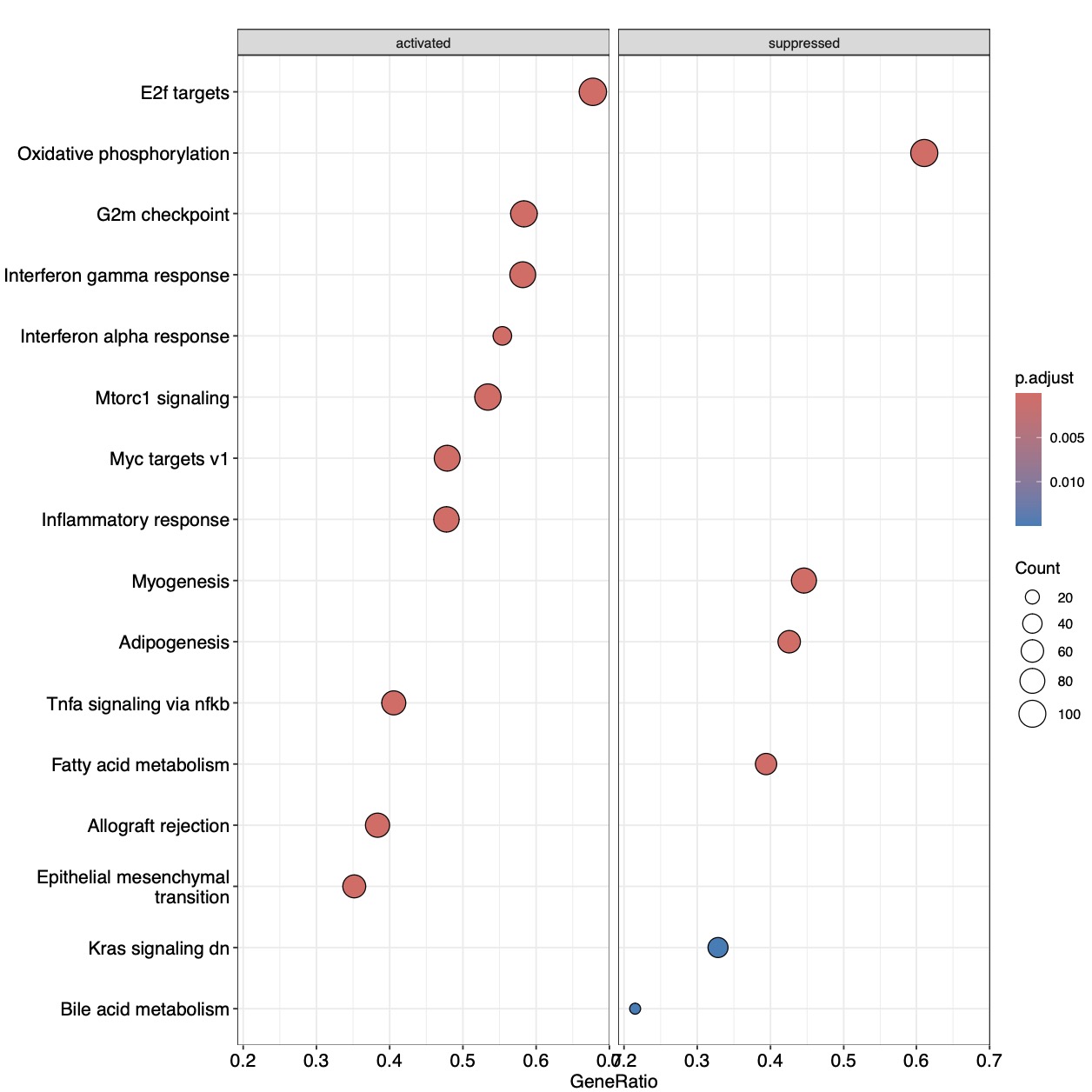
GSE13601

GSE9844

这里我们将GSEA中的激活和抑制基因通路富集分别做了展示

三、韦恩图分析—两组数据

1.输入数据

#为了连续性，从头开始
rm(list = ls())
GSE9844 <- read.csv("GSE9844-degs.csv", header = T, check.names = T)
GSE13601 <- read.csv("GSE13601-degs.csv", header = T, check.names = T)

2.提取差异基因

Degs_GSE9844 <- GSE9844[!GSE9844$change == "stable",]
Degs_GSE13601 <- GSE13601[!GSE13601$change == "stable",]

up_GSE9844 <- GSE9844[GSE9844$change == "up",]
down_GSE9844 <- GSE9844[GSE9844$change == "down",]

up_GSE13601 <- GSE13601[GSE13601$change == "up",]
down_GSE13601 <- GSE13601[GSE13601$change == "down",]

3.二元韦恩图绘制-total

#UP和Down基因的韦恩图需要微调参数
Degs_total = list(GSE9844 = Degs_GSE9844$symbol,
                  GSE13601 = Degs_GSE13601$symbol)

#韦恩图绘制
c <- c("#c9e3f1","#eda587") #用Snipaste软件检测
  
#韦恩图绘制
library(patchwork)
library(VennDiagram)
# 开启PNG设备，设置文件名、宽度、高度和分辨率
png(filename = "Degs_total.png", width = 2000, height = 2000, res = 300)
venn.diagram(Degs_total,
             scaled = F, # 根据比例显示大小
             alpha= 0.5, #透明度
             lwd=1,
             lty=1,
             col= "transparent", 
             label.col ='black' , 
             cex = 2, # 数字大小
             fontface = "bold",  # 字体粗细；加粗bold
             fill=c, 
             category.names = c("GSE9844","GSE13601") , #标签名
             cat.dist = 0.02, 
             cat.pos = -180, 
             cat.cex = 2, #标签字体大小
             cat.fontface = "bold",  # 标签字体加粗
             cat.col='black' ,  
             cat.default.pos = "outer",  # 标签位置,
             main = "Degs_total_Venn",
             main.cex = 2,
             output=TRUE,
             filename='Degs_total.png',# 文件保存
             imagetype="png",  
             resolution = 400,  # 分辨率
             compression = "lzw"# 压缩算法
)
dev.off()

Up基因交集

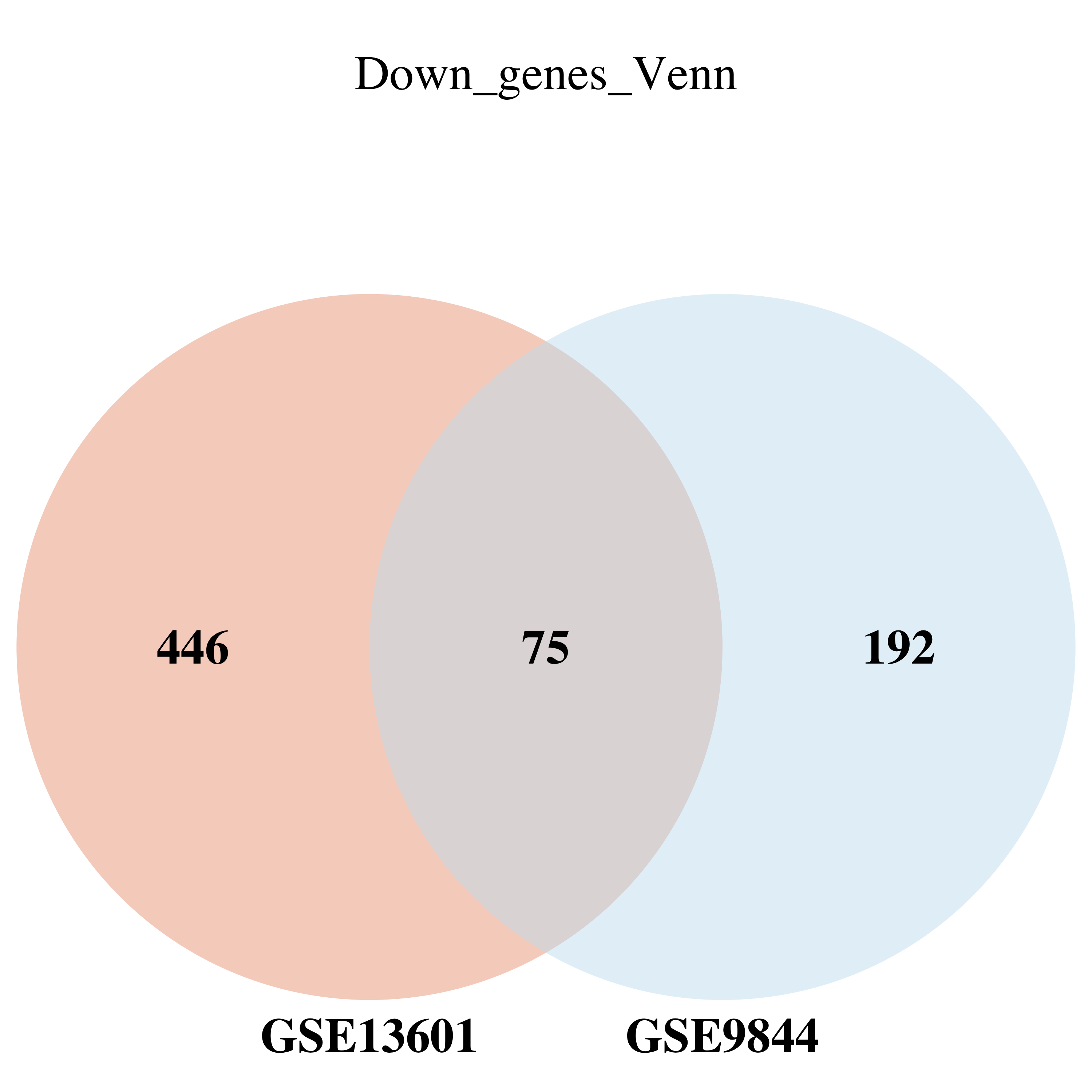
Down基因交集

四、jaccard相似性指数，Pearson和Spearman相关系数，差异基因列表重叠分析，回归分析分析

1.导入差异基因文档

#为了连续性，从头开始
rm(list = ls())
GSE9844 <- read.csv("GSE9844-degs.csv", header = T, check.names = T)
GSE13601 <- read.csv("GSE13601-degs.csv", header = T, check.names = T)

2.提取差异基因

Degs_GSE9844 <- GSE9844[!GSE9844$change == "stable",]
Degs_GSE13601 <- GSE13601[!GSE13601$change == "stable",]

3.Jaccard相似性指数

# 手动计算 或 proxy包可计算jaccard相似性指数
# 假设这些是你的基因符号向量
symbols_GSE13601 <- Degs_GSE13601$symbol
symbols_GSE9844 <- Degs_GSE9844$symbol
# 创建全集
all_symbols <- union(symbols_GSE13601, symbols_GSE9844)
# 创建逻辑向量
vector_GSE13601 <- all_symbols %in% symbols_GSE13601
vector_GSE9844 <- all_symbols %in% symbols_GSE9844
# 组合为矩阵
data_matrix <- rbind(vector_GSE13601, vector_GSE9844)

#手动计算
# 计算交集和并集的大小
intersection_size <- sum(vector_GSE13601 & vector_GSE9844)
union_size <- sum(vector_GSE13601 | vector_GSE9844)
# 计算 Jaccard 相似性指数
jaccard_index <- intersection_size / union_size
print(jaccard_index)

#proxy包实现
library(proxy)
# 计算 Jaccard 距离
jaccard_distance <- proxy::dist(data_matrix, method = "Jaccard")
# 距离转相似性（距离越小，相似性越高）
jaccard_similarity <- 1 - as.numeric(jaccard_distance)
print(jaccard_similarity)
# jaccard = 0.1203993

最后得到jaccard值为0.1203993

4.Pearson和Spearman相关系数

#获取交集基因
common_genes <- intersect(Degs_GSE9844$symbol, Degs_GSE13601$symbol)
# 筛选共同的交集基因及其它信息
Degs1 <- Degs_GSE13601[Degs_GSE13601$symbol %in% common_genes, ]
Degs2 <- Degs_GSE9844[Degs_GSE9844$symbol %in% common_genes, ]
# 确保数据按基因符号排序
Degs1 <- Degs1[order(Degs1$symbol), ]
Degs2 <- Degs2[order(Degs2$symbol), ]
identical(Degs1$symbol,Degs2$symbol)

# 计算 Pearson 相关系数
pearson_correlation <- cor(Degs1$logFC, Degs2$logFC,method = c("pearson"))
print(paste("Pearson correlation coefficient:", pearson_correlation))
# "Pearson correlation coefficient: 0.891066993607884"

# 计算Spearman秩相关系数
spearman_correlation <- cor(Degs1$logFC, Degs2$logFC,method = c("spearman"))
print(paste("Spearman correlation coefficient:", spearman_correlation))
# "Spearman correlation coefficient: 0.826690280967897"

最后得到Pearson 相关系数为0.891066993607884，Spearman秩相关系数为0.826690280967897

5.差异基因列表重叠分析

# 大样本采用超几何分布检验
# 在R中，可以使用phyper函数来进行超几何分布检验

# 假设所有已知基因的总数(大概就是这个数2W左右)
total_genes <- 20000
# 计算共有基因数量
common_genes <- length(intersect(Degs_GSE13601$symbol, 
                                 Degs_GSE9844$symbol))
# 进行超几何测试
p_value_hyper <- phyper(common_genes - 1, #共同基因数-1
                        length(Degs_GSE13601$symbol),  #在Degs1中发现的差异基因
                        total_genes - length(Degs_GSE13601$symbol), #总体基因减去Degs1中的差异基因
                        length(Degs_GSE9844$symbol),  #Degs2中发现的差异基因
                        lower.tail = FALSE)
print(paste("P-value from hypergeometric test:", p_value_hyper))
# "P-value from hypergeometric test: 5.94789155387934e-97"
# p值小于0.05时，可以认为这种重叠是统计上显著的，不太可能仅仅是偶然发生


#如果小样本需要用Fisher精确检验
# Fisher精确检验可以用fisher.test函数实现。

#以下是示例代码
# 构建列联表
#overlap <- length(intersect(genes_group1, genes_group2))
#only_group1 <- length(genes_group1) - overlap
#only_group2 <- length(genes_group2) - overlap
#neither <- total_genes - overlap - only_group1 - only_group2

#contingency_table <- matrix(c(overlap, only_group1, only_group2, neither), 
                        #     nrow = 2, 
                         #    byrow = TRUE)

# 进行Fisher精确检验
#fisher_test_result <- fisher.test(contingency_table)
#print(paste("P-value from Fisher's Exact Test:", #fisher_test_result$p.value))

最后得到超几何分布的值为5.94789155387934e-97

6.回归分析

#获取交集基因
common_genes <- intersect(Degs_GSE9844$symbol, Degs_GSE13601$symbol)
# 筛选共同的交集基因及其它信息
Degs1 <- Degs_GSE13601[Degs_GSE13601$symbol %in% common_genes, ]
Degs2 <- Degs_GSE9844[Degs_GSE9844$symbol %in% common_genes, ]
# 确保数据按基因符号排序
Degs1 <- Degs1[order(Degs1$symbol), ]
Degs2 <- Degs2[order(Degs2$symbol), ]
identical(Degs1$symbol,Degs2$symbol)

# 合并数据集
merged_data <- merge(Degs1, Degs2, by = "symbol")

# 拟合线性模型
model <- lm(logFC.x~ logFC.y, data = merged_data)
# 查看模型摘要
summary(model)

library(ggplot2)
# 绘制散点图和回归线
p <- ggplot(merged_data, aes(x = logFC.x, y = logFC.y)) +
     geom_point() +
     geom_smooth(method = "lm", color = "blue") +
     labs(x = "log2FC from Degs1", 
          y = "log2FC from Degs2", 
          title = "Regression Analysis Between Two Gene Sets") +
     theme_minimal()

print(p)

小结：通过多种工具发现对不同数据中获得的差异基因分析会得到具有差异的结果，因此这也提示我们在进行分析的时候需要通过多种手段综合判断。

致谢：感谢曾老师，小洁老师以及生信技能树团队全体成员（部分代码来源：生信技能树马拉松和数据挖掘课程）。

注：若对内容有疑惑或者发现有明确错误的，请联系后台(希望多多交流)。更多内容可见公众号：生信方舟