三角测量计算点的三维坐标

最新推荐文章于 2025-03-25 10:48:28 发布

@way

最新推荐文章于 2025-03-25 10:48:28 发布

阅读量6.4k

点赞数 11

分类专栏：机器视觉文章标签：计算机视觉

本文链接：https://blog.csdn.net/zhaitianyong/article/details/111168657

版权

机器视觉专栏收录该内容

9 篇文章

订阅专栏

三角测量（triangulation), 就是在不同的姿态下观察同一个对象，根据图像上的同名点的像素坐标，计算对象的三维坐标。

在双目视觉中，分左右相机，同时可以获得左视图和右视图，根据匹配的同名点和左右相机的投影矩阵，就可以计算出匹配同名点的世界坐标。
在这里插入图片描述
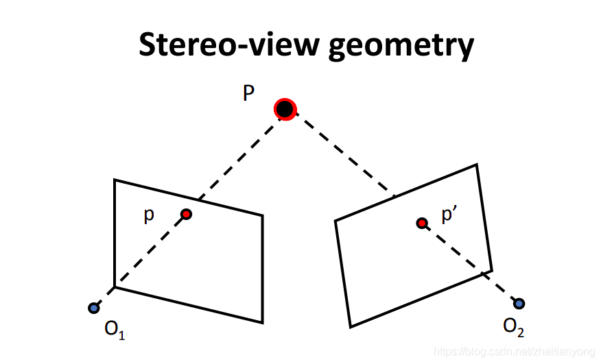
如图： O1和O2相机的投影的像素点为p， p’；P为世界坐标点的齐次坐标。
首先对两个相机进行标定，并获得投影矩阵分别是T1 和 T2， T1和T2的大小为3x4的矩阵。

$\left[\begin{matrix} u \\ v \\ 1 \end{matrix}\right] p^{'} = \left[\begin{matrix} u ^{'}\\ v ^{'}\\ 1 \end{matrix}\right]$
根据：

$s_1p = T_1P \\ s_2p'=T_2P$

s1和s2 为尺度。把T1分解成行向量T11、T12、T13。
$s_1\left[\begin{matrix} u \\ v \\ 1 \end{matrix}\right] = \left[\begin{matrix} T_{11} \\ T_{12} \\ T_{13} \end{matrix}\right]P$
分解
$s_1v=T_{11}P \\ s_1u = T_{12}P \\ s_1 = T_{13}P \\$
把第三式带入，消去 $s_1$
$vT_{13}P=T_{11}P \\ u T_{13}P= T_{12}P \\ =>\\ (vT_{13}- T_{11})P=0 \\ (uT_{13}-T_{12})P=0\\$
可以看出，一对点可以有4个方程，P有3个未知数。可以把等式写成AP=0形式。
即：
$\left[\begin{matrix} vT_{13}- T_{11} \\ uT_{13}-T_{12}\\ v^{'}T_{23}- T_{21} \\ u^{'}T_{23}-T_{22} \end{matrix}\right]P=0$

然后对A进行SVD分解，最小二乘法就可以计算出P。

代码实现：


/**
 * 
 * @param T1 相机O1的投影矩阵
 * @param T2 相机O2的投影矩阵
 * @param p1 相机O1的图像的像素点
 * @param p2 相机O2的图像的像素点
 * @param out 输出的三维坐标
 */
void triangulatePoint(Matrix<double, 3, 4>& T1, Matrix<double, 3, 4>& T2, Vector2d& p1, Vector2d&p2, Vector3d& out){
    // 构建Ax = 0;
    Matrix<double, 4, 4> A;
    A.row(0) = p1(0)*T1.row(2) - T1.row(0);
    A.row(1) = p1(1)*T1.row(2) - T1.row(1);
    A.row(2) = p2(0)*T2.row(2) - T2.row(0);
    A.row(3) = p2(1)*T2.row(2) - T2.row(1);

    // SVD 分解
    Eigen::JacobiSVD<MatrixXd> solver(A, Eigen::ComputeFullU|Eigen::ComputeThinV);
    MatrixXd V = solver.matrixV();
    VectorXd X = V.rightCols(1);

    out[0] = X(0)/X(3);
    out[1] = X(1)/X(3);
    out[2] = X(2)/X(3);
}

OpenCV库，也已经实现了cv::triangulatePoints
这里也对其进行调用

void triangulateByOpenCV(Matrix<double, 3, 4>& T1, Matrix<double, 3, 4>& T2, Vector2d& p1, Vector2d&p2, Vector3d& out){

    Mat T_mat1, T_mat2;
    cv::eigen2cv(T1, T_mat1);
    cv::eigen2cv(T2, T_mat2);


    std::vector<Point2d> p1s,p2s;
    p1s.push_back(Point2d(p1.x(), p1.y()));
    p2s.push_back(Point2d(p2.x(), p2.y()));


    /*
     *  @param projMatr1 3x4 projection matrix of the first camera.
        @param projMatr2 3x4 projection matrix of the second camera.
        @param projPoints1 2xN array of feature points in the first image. In case of c++ version it can
        be also a vector of feature points or two-channel matrix of size 1xN or Nx1.
        @param projPoints2 2xN array of corresponding points in the second image. In case of c++ version
        it can be also a vector of feature points or two-channel matrix of size 1xN or Nx1.
        @param points4D 4xN array of reconstructed points in homogeneous coordinates.
     *
     */
    Mat pts_4d;
    cv::triangulatePoints(T_mat1, T_mat2, p1s, p2s, pts_4d);

    Mat X = pts_4d.col(0);
    X /=X.at<double>(3,0);

    out[0] = X.at<double>(0, 0);
    out[1] = X.at<double>(1, 0);
    out[2] = X.at<double>(2, 0);

}

对两个函数进行测试，数据来自网络。


int main(){

    Matrix<double, 3, 4> T1, T2;
    T1(0, 0) = 0.919653;    T1(0, 1)=-0.000621866; T1(0, 2)= -0.00124006; T1(0, 3) = 0.00255933;
    T1(1, 0) = 0.000609954; T1(1, 1)=0.919607    ; T1(1, 2)= -0.00957316; T1(1, 3) = 0.0540753;
    T1(2, 0) = 0.00135482;  T1(2, 1) =0.0104087  ; T1(2, 2)= 0.999949;    T1(2, 3) = -0.127624;

    T2(0, 0) = 0.920039;    T2(0, 1)=-0.0117214;  T2(0, 2) = 0.0144298;   T2(0, 3)   = 0.0749395;
    T2(1, 0) = 0.0118301;   T2(1, 1)=0.920129  ;  T2(1, 2) = -0.00678373; T2(1, 3) = 0.862711;
    T2(2, 0) = -0.0155846;  T2(2, 1) =0.00757181; T2(2, 2) = 0.999854 ;   T2(2, 3)   = -0.0887441;

    Vector2d p1, p2;
    p1(0) = 0.289986; p1(1) = -0.0355493;
    p2(0) = 0.316154; p2(1) =  0.0898488;



    Vector3d out1, out2;
    triangulatePoint(T1, T2, p1, p2, out1);

    triangulateByOpenCV(T1, T2, p1, p2, out2);

    std::cout<< "result 1 >> " << out1.transpose() << std::endl;
    std::cout<< "result 2 >> " << out2.transpose() << std::endl;

    return 0;
}

两个函数输出的结果一致：

result 1 >>   2.14598 -0.250569   6.92321
result 2 >>   2.14598 -0.250569   6.92321

参考：
http://users.cecs.anu.edu.au/~hartley/Papers/triangulation/triangulation.pdf
http://vision.stanford.edu/teaching/cs231a_autumn1112/lecture/lecture10_multi_view_cs231a_old.pdf