无人驾驶汽车系统入门（七）——基于传统计算机视觉的车道线检测(2)

最新推荐文章于 2023-04-25 17:14:50 发布

置顶 AdamShan

最新推荐文章于 2023-04-25 17:14:50 发布

阅读量2.9w

点赞数 33

分类专栏：无人驾驶汽车专题无人驾驶汽车系统入门文章标签：计算机视觉弯曲车道线检测车道线检测

本文链接：https://blog.csdn.net/adamshan/article/details/78733302

版权

无人驾驶汽车专题同时被 2 个专栏收录

32 篇文章 1005 订阅

订阅专栏

无人驾驶汽车系统入门

32 篇文章 1102 订阅

订阅专栏

无人驾驶汽车系统入门（七）——基于传统计算机视觉的车道线检测(2)

原创不易，转载请注明来源：http://blog.csdn.net/adamshan/article/details/78733302

接上文，在获得ROI（透视变换）以后，我们对得到的“鸟瞰图”应用色彩阈值化和梯度阈值化，以得到鸟瞰图中“可能为”车道线的像素然后再使用滑动窗口来确定车道线的多项式系数，下面我们来具体讨论这两个步骤。

边缘检测

车道线的一个主要的特征就是它可以看作图像中的边缘（Edge），因此我们可以使用一定的 边缘检测(Edge detection) 算法将之从原图像中提取出来。边缘检测的结果就是标识出了数字图像中亮度变化明显的点。有许多用于边缘检测的方法，他们大致可分为两类：基于搜索和基于零交叉。

基于搜索的边缘检测方法首先计算边缘强度，通常用一阶导数表示，例如梯度模; 然后，用计算估计边缘的局部方向，通常采用梯度的方向，并利用此方向找到局部梯度模的最大值。
基于零交叉的方法找到由图像得到的二阶导数的零交叉点来定位边缘.通常用拉普拉斯算子或非线性微分方程的零交叉点。

本文介绍一种基于亮度的一阶导数的方法，或者说，基于原始图像的亮度的梯度的算法。我们使用 索贝尔算子（Sobel operator） 来计算图像中的边缘，该算子包含两组 $3\times3$ 的矩阵，分别为横向和纵向，将之与图像作平面卷积，即可分别得出横向及纵向的亮度差分近似值。如果以 $A$ 代表原始图像， $G_x$ 及 $G_y$ 分别代表经横向及纵向边缘检测的图像，其公式如下:

G x = ⎡ ⎣ ⎢ ⎢ - 1 - 2 - 1 000 + 1 + 2 + 1 ⎤ ⎦ ⎥ ⎥ * A

$G_x = \left[ \begin{array}{cc} -1 & 0 & +1 \\ -2 & 0 & +2 \\ -1 & 0 & +1 \end{array} \right] * A$

G y = ⎡ ⎣ ⎢ ⎢ - 1 0 + 1 - 2 0 + 2 - 1 0 + 1 ⎤ ⎦ ⎥ ⎥ * A

$G_y = \left[ \begin{array}{cc} -1 & -2 & -1 \\ 0 & 0 & 0 \\ +1 & +2 & +1 \end{array} \right] * A$

在OpenCV中，可以使用 cv2.Sobel() 方法来指定，我们来看一下横向和纵向的索贝尔算子检测的边缘的区别，这里我们使用拉普拉斯算子作为参照：

import cv2
import numpy as np
from matplotlib import pyplot as plt

img = cv2.imread('test_images/shudu.jpeg', 0)

laplacian = cv2.Laplacian(img, cv2.CV_64F)
sobelx = cv2.Sobel(img, cv2.CV_64F, 1, 0, ksize=3)
sobely = cv2.Sobel(img, cv2.CV_64F, 0, 1, ksize=3)

plt.subplot(2, 2, 1), plt.imshow(img, cmap='gray')
plt.title('Original'), plt.xticks([]), plt.yticks([])
plt.subplot(2, 2, 2), plt.imshow(laplacian, cmap='gray')
plt.title('Laplacian'), plt.xticks([]), plt.yticks([])
plt.subplot(2, 2, 3), plt.imshow(sobelx, cmap='gray')
plt.title('Sobel X'), plt.xticks([]), plt.yticks([])
plt.subplot(2, 2, 4), plt.imshow(sobely, cmap='gray')
plt.title('Sobel Y'), plt.xticks([]), plt.yticks([])

plt.show()

检测的结果：

这里写图片描述

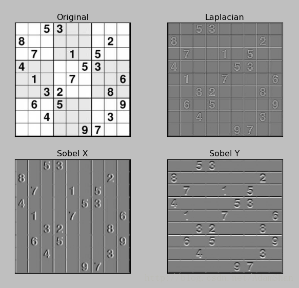
不难看出， $x$ 方向的索贝尔算子倾向于检测垂直方向的边缘，而 $y$ 方向的索贝尔算子则倾向于检测水平的边缘，而在车道线检测问题中，我们关注的对象（车道线）往往是垂直方向的线，同时我们希望过滤到一些水平方向的线，所以在本实例中，我们采用 $x$ 方向的索贝尔算子。

通过使用索贝尔算子做两个方向的卷积，我们可以得到图像的每一个像素的横向及纵向 梯度近似值 ，更近一步，我们可以结合这两个近似值计算梯度的大小：

G = G 2 x + G 2 y ‾ ‾ ‾ ‾ ‾ ‾ ‾ ‾ \sqrt

$G = \sqrt{G_x^2 + G_y^2}$

然后可用以下公式计算梯度方向:

Θ = arctan (G y G x)

$\Theta = \arctan \left( \frac{G_y}{G_x} \right)$

我们分别使用OpenCV实现以上的内容：

def abs_sobel_thresh(img, sobel_kernel=3, orient='x', thresh=(0, 255)):
    gray = cv2.cvtColor(img, cv2.COLOR_RGB2GRAY)
    if orient == 'x':
        sobel = cv2.Sobel(gray, cv2.CV_64F, 1, 0, ksize=sobel_kernel)
    else:
        sobel = cv2.Sobel(gray, cv2.CV_64F, 0, 1, ksize=sobel_kernel)
    abs_sobel = np.absolute(sobel)
    scaled_sobel = np.uint8(255 * abs_sobel / np.max(abs_sobel))
    sxbinary = np.zeros_like(scaled_sobel)
    sxbinary[(scaled_sobel >= thresh[0]) & (scaled_sobel <= thresh[1])] = 1
    return sxbinary


def mag_thresh(img, sobel_kernel=3, mag_thresh=(0, 255)):
    # Convert to grayscale
    gray = cv2.cvtColor(img, cv2.COLOR_RGB2GRAY)
    # Take both Sobel x and y gradients
    sobelx = cv2.Sobel(gray, cv2.CV_64F, 1, 0, ksize=sobel_kernel)
    sobely = cv2.Sobel(gray, cv2.CV_64F, 0, 1, ksize=sobel_kernel)
    # Calculate the gradient magnitude
    gradmag = np.sqrt(sobelx**2 + sobely**2)
    # Rescale to 8 bit
    scale_factor = np.max(gradmag)/255
    gradmag = (gradmag/scale_factor).astype(np.uint8)
    # Create a binary image of ones where threshold is met, zeros otherwise
    binary_output = np.zeros_like(gradmag)
    binary_output[(gradmag >= mag_thresh[0]) & (gradmag <= mag_thresh[1])] = 1

    # Return the binary image
    return binary_output


def dir_threshold(img, sobel_kernel=3, thresh=(0, np.pi/2)):
    # Grayscale
    gray = cv2.cvtColor(img, cv2.COLOR_RGB2GRAY)
    # Calculate the x and y gradients
    sobelx = cv2.Sobel(gray, cv2.CV_64F, 1, 0, ksize=sobel_kernel)
    sobely = cv2.Sobel(gray, cv2.CV_64F, 0, 1, ksize=sobel_kernel)
    # Take the absolute value of the gradient direction,
    # apply a threshold, and create a binary image result
    absgraddir = np.arctan2(np.absolute(sobely), np.absolute(sobelx))
    binary_output =  np.zeros_like(absgraddir)
    binary_output[(absgraddir >= thresh[0]) & (absgraddir <= thresh[1])] = 1

    # Return the binary image
    return binary_output

分别对上一篇文章中的鸟瞰图进行边缘检测：

ksize = 9 # Choose a larger odd number to smooth gradient measurements

# Apply each of the thresholding functions
gradx = abs_sobel_thresh(wrap_img, orient='x', sobel_kernel=3, thresh=(20, 255))

mag_binary = mag_thresh(wrap_img, sobel_kernel=3, mag_thresh=(30, 100))
dir_binary = dir_threshold(wrap_img, sobel_kernel=15, thresh=(0.7, 1.3))

# Plot the result
f, axs = plt.subplots(2, 2, figsize=(16, 9))
f.tight_layout()
axs[0, 0].imshow(wrap_img)
axs[0, 0].set_title('Original Image', fontsize=18)
axs[0, 1].imshow(gradx, cmap='gray')
axs[0, 1].set_title('Sobel_x_filter', fontsize=18)
axs[1, 0].imshow(dir_binary, cmap='gray')
axs[1, 0].set_title('Dir_threshold', fontsize=18)
axs[1, 1].imshow(mag_binary, cmap='gray')
axs[1, 1].set_title('Mag_threshold', fontsize=18)
plt.subplots_adjust(left=0., right=1, top=0.9, bottom=0.)
plt.show()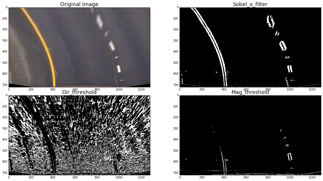

这里写图片描述

不难看出，x方向的索贝尔算子取得了最好的效果，同时，梯度方向也为车道线像素选取提供了一定的参考。

色彩阈值化

检测车道线的另一个依据就是车道线的颜色特征，一般来说，车道线只有两种颜色：白色和黄色，所以我们可以在 RGB 色彩空间(Color Space) 对这两种颜色进行过滤从而提取出车道线的像素。

色彩空间：使用一组值（通常使用三个、四个值或者颜色成分）表示颜色方法的抽象数学模型。有利用原色相混的比例表示的色彩空间，如 RGB (Red, Green, Blue) 颜色空间; 也有利用不同的概念表示的色彩空间,如 HSV (色相 hue, 饱和度 saturation, 明度 value) 以及 HSL (色相 hue，饱和度 saturation，亮度 lightness/luminance) 。

在OpenCV中，RGB三通道的图像的读取 cv2.imread() 的结果是以 BGR 顺序排列的，而在使用matplotlib的 plt.imread() 时，读取的通道排列顺序则为 RGB 。因此此处应当注意区别。

RGB阈值化处理

我们在RGB色彩空间对黄色和白色进行过滤，得到参考的像素：

def r_select(img, thresh=(200, 255)):
    R = img[:,:,0]
    binary = np.zeros_like(R)
    binary[(R > thresh[0]) & (R <= thresh[1])] = 1
    return binary

def color_mask(hsv,low,high):
    # Return mask from HSV
    mask = cv2.inRange(hsv, low, high)
    return mask

def apply_color_mask(hsv,img,low,high):
    # Apply color mask to image
    mask = cv2.inRange(hsv, low, high)
    res = cv2.bitwise_and(img,img, mask= mask)
    return res

def apply_yellow_white_mask(img):
    image_HSV = cv2.cvtColor(img,cv2.COLOR_RGB2HSV)
    yellow_hsv_low  = np.array([ 0,  100,  100])
    yellow_hsv_high = np.array([ 80, 255, 255])
    white_hsv_low  = np.array([ 0,   0,   160])
    white_hsv_high = np.array([ 255,  80, 255])
    mask_yellow = color_mask(image_HSV,yellow_hsv_low,yellow_hsv_high)
    mask_white = color_mask(image_HSV,white_hsv_low,white_hsv_high)
    mask_YW_image = cv2.bitwise_or(mask_yellow,mask_white)
    return mask_YW_image

r_binary = r_select(wrap_img, thresh=(220, 255))
yw_binary = apply_yellow_white_mask(wrap_img)
# Plot the result
f, axs = plt.subplots(1, 2, figsize=(16, 9))
f.tight_layout()
axs[0].imshow(r_binary, cmap='gray')
axs[0].set_title('R filter', fontsize=18)
axs[1].imshow(yw_binary, cmap='gray')
axs[1].set_title('Yellow white filter', fontsize=18)
plt.subplots_adjust(left=0., right=1, top=0.9, bottom=0.)
plt.show()

效果：

这里写图片描述

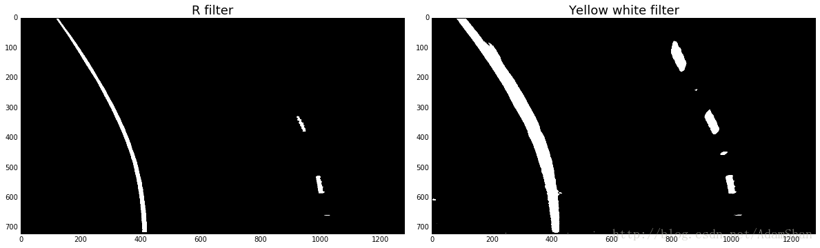
上面的代码中，R filter是在Red通道上设置合适的阈值，就能够对黄色和白色的导线进行过滤，而Yellow white filter则直接对三个通道设置一定的阈值，通过组合（and操作）来获得最优的过滤效果，RGB颜色阈值化虽然能够在正常光线条件下很好的过滤出道线像素，但是在复杂环境光的情况下性能并不稳定。下面我们进一步探索颜色阈值化，看看在 HLS 色彩空间的阈值化效果。

HLS 阈值化处理

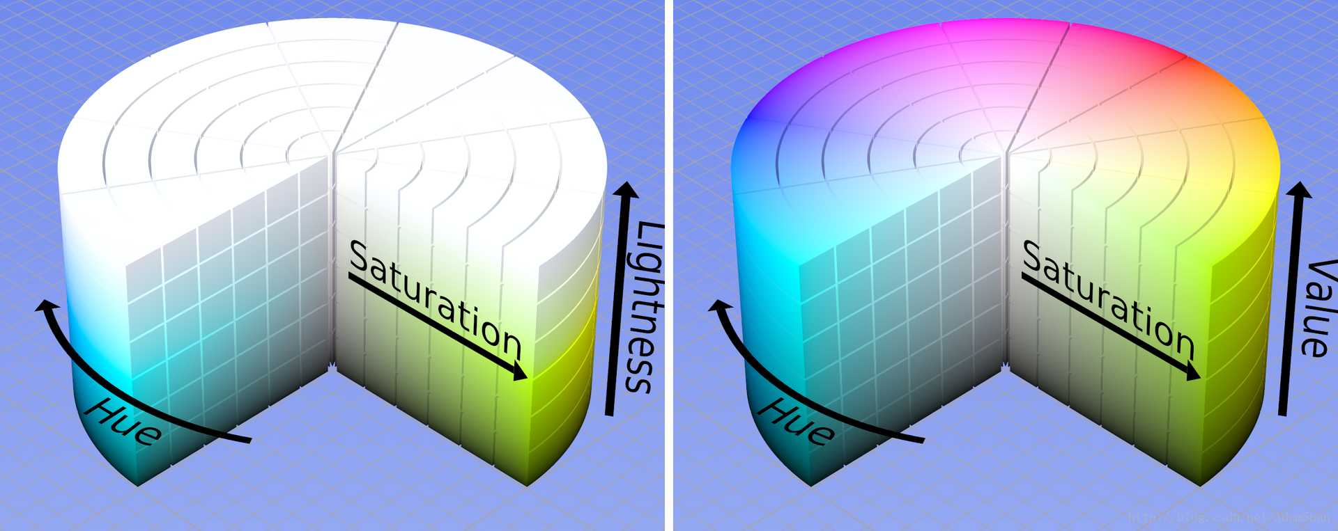
下图是 HLS 色彩空间和 HSV 色彩空间的可视化比较。HLS和HSV都是一种将RGB色彩模型中的点在圆柱坐标系中的表示法。这两种表示法试图做到比RGB基于笛卡尔坐标系的几何结构更加直观。HLS即色相、亮度、饱和度。在本文中，我们重点探讨应用HLS的色彩阈值化于车道线检测。在OpenCV中，我可以直接使用 cv2.cvtColor() 方法将图像从RGB色彩空间转换到HLS色彩空间。

这里写图片描述

我们对HLS色彩空间的三个通道分别对车道线进行阈值化处理：

def hls_select(img, channel='S', thresh=(90, 255)):
    # 1) Convert to HLS color space
    # 2) Apply a threshold to the S channel
    # 3) Return a binary image of threshold result
    hls = cv2.cvtColor(img, cv2.COLOR_RGB2HLS)
    if channel == 'S':
        X = hls[:, :, 2]
    elif channel == 'H':
        X = hls[:, :, 0]
    elif channel == 'L':
        X = hls[:, :, 1]
    else:
        print('illegal channel !!!')
        return
    binary_output = np.zeros_like(X)
    binary_output[(X > thresh[0]) & (X <= thresh[1])] = 1
    return binary_output

对鸟瞰图测试阈值：

l_binary = hls_select(wrap_img, channel='L', thresh=(100, 200))
s_binary = hls_select(wrap_img, channel='S', thresh=(100, 255))
h_binary = hls_select(wrap_img, channel='H', thresh=(100, 255))
f, axs = plt.subplots(2, 2, figsize=(16, 9))
f.tight_layout()
axs[0, 0].imshow(wrap_img)
axs[0, 0].set_title('Original Image', fontsize=18)
axs[0, 1].imshow(h_binary, cmap='gray')
axs[0, 1].set_title('H channal filter', fontsize=18)
axs[1, 0].imshow(s_binary, cmap='gray')
axs[1, 0].set_title('S channal filter', fontsize=18)
axs[1, 1].imshow(l_binary, cmap='gray')
axs[1, 1].set_title('L channal filter', fontsize=18)
plt.subplots_adjust(left=0., right=1, top=0.9, bottom=0.)
plt.show()

结果如下：

这里写图片描述

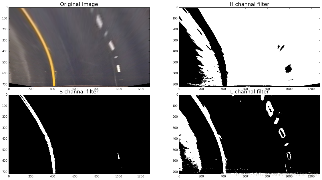
粗略看来，通过组合H和S的阈值化可以获得良好的检测效果。

组合梯度和色彩过滤车道线像素

最理想的自然是通过组合以上的方法来获得对车道线最理想的提取，这种组合方法有很多，没有一个固定的模式，通过组合梯度和色彩过滤器，可以获得一个相对稳定的车道线提取方法，最理想的状态就是我们的组合过滤器能够尽可能少受到环境光，道路背景色以及其他车辆的影响，再次我们给出一个参考的组合方法：

def combine_filters(img):
    gradx = abs_sobel_thresh(img, orient='x', sobel_kernel=3, thresh=(20, 255))
    l_binary = hls_select(img, channel='L', thresh=(100, 200))
    s_binary = hls_select(img, channel='S', thresh=(100, 255))
    yw_binary = apply_yellow_white_mask(wrap_img)
    yw_binary[(yw_binary !=0)] = 1
    combined_lsx = np.zeros_like(gradx)
    combined_lsx[((l_binary == 1) & (s_binary == 1) | (gradx == 1) | (yw_binary == 1))] = 1
    return combined_lsx

binary = combine_filters(wrap_img)
f, axs = plt.subplots(1, 2, figsize=(16, 9))
f.tight_layout()
axs[0].imshow(wrap_img)
axs[0].set_title('Original', fontsize=18)
axs[1].imshow(binary, cmap='gray')
axs[1].set_title('combine filters', fontsize=18)
plt.subplots_adjust(left=0., right=1, top=0.9, bottom=0.)
plt.show()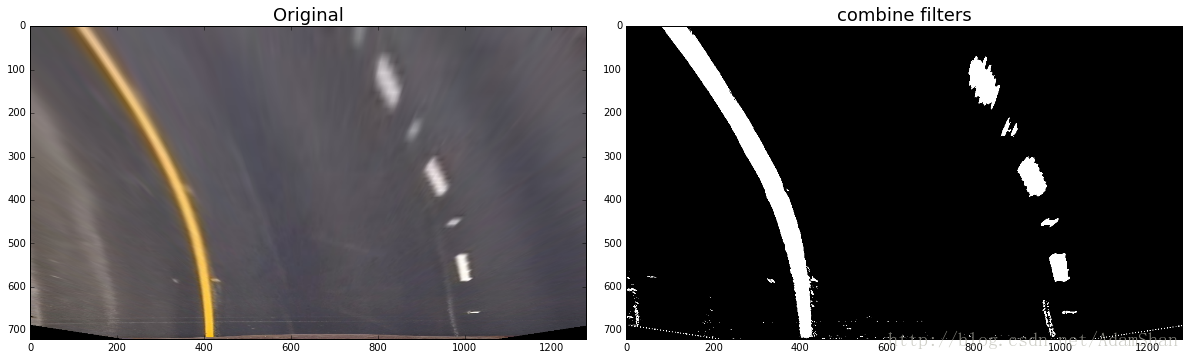

这里写图片描述

在提取完车道线像素以后，我们用两条曲线来拟合这些像素，在做拟合这一步操作之前，我们首先得确定哪些像素是车道线的，哪些不是，这里我们使用滑动窗口的方法。

滑动窗口与多项式拟合

滑动窗口的代码如下：

def find_line_fit(img, nwindows=9, margin=100, minpix=50):
    histogram = np.sum(img[img.shape[0]//2:,:], axis=0)
    # Create an output image to draw on and  visualize the result
    out_img = np.dstack((img, img, img)) * 255
    # Find the peak of the left and right halves of the histogram
    # These will be the starting point for the left and right lines
    midpoint = np.int(histogram.shape[0]/2)
    leftx_base = np.argmax(histogram[:midpoint])
    rightx_base = np.argmax(histogram[midpoint:]) + midpoint

    # Set height of windows
    window_height = np.int(img.shape[0]/nwindows)
    # Identify the x and y positions of all nonzero pixels in the image
    nonzero = img.nonzero()
    nonzeroy = np.array(nonzero[0])
    nonzerox = np.array(nonzero[1])
    # Current positions to be updated for each window
    leftx_current = leftx_base
    rightx_current = rightx_base
    # Create empty lists to receive left and right lane pixel indices
    left_lane_inds = []
    right_lane_inds = []

    # Step through the windows one by one
    for window in range(nwindows):
        # Identify window boundaries in x and y (and right and left)
        win_y_low = img.shape[0] - (window+1)*window_height
        win_y_high = img.shape[0] - window*window_height
        win_xleft_low = leftx_current - margin
        win_xleft_high = leftx_current + margin
        win_xright_low = rightx_current - margin
        win_xright_high = rightx_current + margin
        # Draw the windows on the visualization image
        cv2.rectangle(out_img,(win_xleft_low,win_y_low),(win_xleft_high,win_y_high),
        (0,255,0), 2)
        cv2.rectangle(out_img,(win_xright_low,win_y_low),(win_xright_high,win_y_high),
        (0,255,0), 2)
        # Identify the nonzero pixels in x and y within the window
        good_left_inds = ((nonzeroy >= win_y_low) & (nonzeroy < win_y_high) &
        (nonzerox >= win_xleft_low) &  (nonzerox < win_xleft_high)).nonzero()[0]
        good_right_inds = ((nonzeroy >= win_y_low) & (nonzeroy < win_y_high) &
        (nonzerox >= win_xright_low) &  (nonzerox < win_xright_high)).nonzero()[0]
        # Append these indices to the lists
        left_lane_inds.append(good_left_inds)
        right_lane_inds.append(good_right_inds)
        # If you found > minpix pixels, recenter next window on their mean position
        if len(good_left_inds) > minpix:
            leftx_current = np.int(np.mean(nonzerox[good_left_inds]))
        if len(good_right_inds) > minpix:
            rightx_current = np.int(np.mean(nonzerox[good_right_inds]))

    # Concatenate the arrays of indices
    left_lane_inds = np.concatenate(left_lane_inds)
    right_lane_inds = np.concatenate(right_lane_inds)

    # Extract left and right line pixel positions
    leftx = nonzerox[left_lane_inds]
    lefty = nonzeroy[left_lane_inds]
    rightx = nonzerox[right_lane_inds]
    righty = nonzeroy[right_lane_inds]

    # to plot
    out_img[nonzeroy[left_lane_inds], nonzerox[left_lane_inds]] = [255, 0, 0]
    out_img[nonzeroy[right_lane_inds], nonzerox[right_lane_inds]] = [0, 0, 255]

    # Fit a second order polynomial to each
    left_fit = np.polyfit(lefty, leftx, 2)
    right_fit = np.polyfit(righty, rightx, 2)
    return left_fit, right_fit, out_img

# Generate x and y values for plotting
def get_fit_xy(img, left_fit, right_fit):
    ploty = np.linspace(0, img.shape[0]-1, img.shape[0])
    left_fitx = left_fit[0]*ploty**2 + left_fit[1]*ploty + left_fit[2]
    right_fitx = right_fit[0]*ploty**2 + right_fit[1]*ploty + right_fit[2]
    return left_fitx, right_fitx, ploty

left_fit, right_fit, out_img = find_line_fit(binary)
left_fitx, right_fitx, ploty = get_fit_xy(binary, left_fit, right_fit)

fig = plt.figure(figsize=(16, 9))
plt.imshow(out_img)
plt.plot(left_fitx, ploty, color='white', linewidth=3.0)
plt.plot(right_fitx, ploty, color='white',  linewidth=3.0)
plt.xlim(0, 1280)
plt.ylim(720, 0)
plt.show()

结果：

这里写图片描述

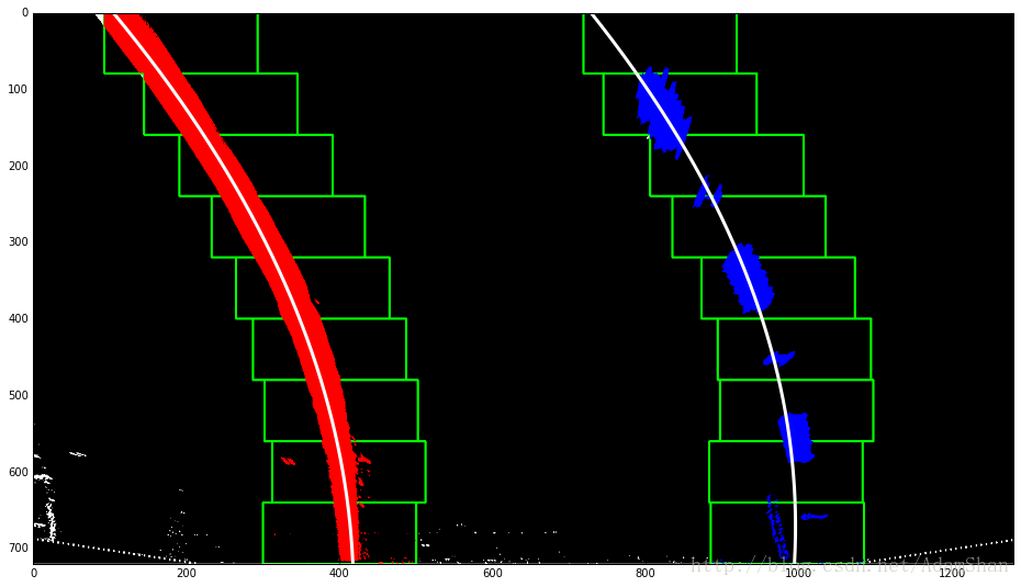
具体来说，为了确定哪些像素属于车道线，首先确定左右两条车道线的大致位置，这一步非常简单，只需要将图片中的像素沿y轴累加，找出图片中间点左右的峰值，即为车道线可能的区域，然后自底向上使用滑动窗口，计算窗口内的不为0的像素点，如果像素点的数量大于某个阈值，那么就以这些点的均值作为下一个滑动窗口的中心。

得到候选的像素以后，使用numpy中的 np.polyfit()方法来拟合这些点，我们使用一个二次多项式来拟合。

拟合的曲线是x关于y的多项式表述，即自变量是y,因变量是x。

还原至原视角

接着在将拟合的曲线使用透视变换还原到原视角：

def project_back(wrap_img, origin_img, left_fitx, right_fitx, ploty, M):
    warp_zero = np.zeros_like(wrap_img).astype(np.uint8)
    color_warp = np.dstack((warp_zero, warp_zero, warp_zero))

    # Recast the x and y points into usable format for cv2.fillPoly()
    pts_left = np.array([np.transpose(np.vstack([left_fitx, ploty]))])
    pts_right = np.array([np.flipud(np.transpose(np.vstack([right_fitx, ploty])))])
    pts = np.hstack((pts_left, pts_right))

    # Draw the lane onto the warped blank image
    cv2.fillPoly(color_warp, np.int_([pts]), (0, 0, 255))

    # Warp the blank back to original image space using inverse perspective matrix (Minv)
    newwarp = perspective_transform(color_warp, M)
    # Combine the result with the original image
    result = cv2.addWeighted(origin_img, 1, newwarp, 0.3, 0)
    return result

M = cv2.getPerspectiveTransform(np.float32(dst_corners), np.float32(src_corners))
result = project_back(binary, test_img, left_fitx, right_fitx, ploty, M)
fig = plt.figure(figsize=(16, 9))
plt.imshow(result)

效果：
这里写图片描述

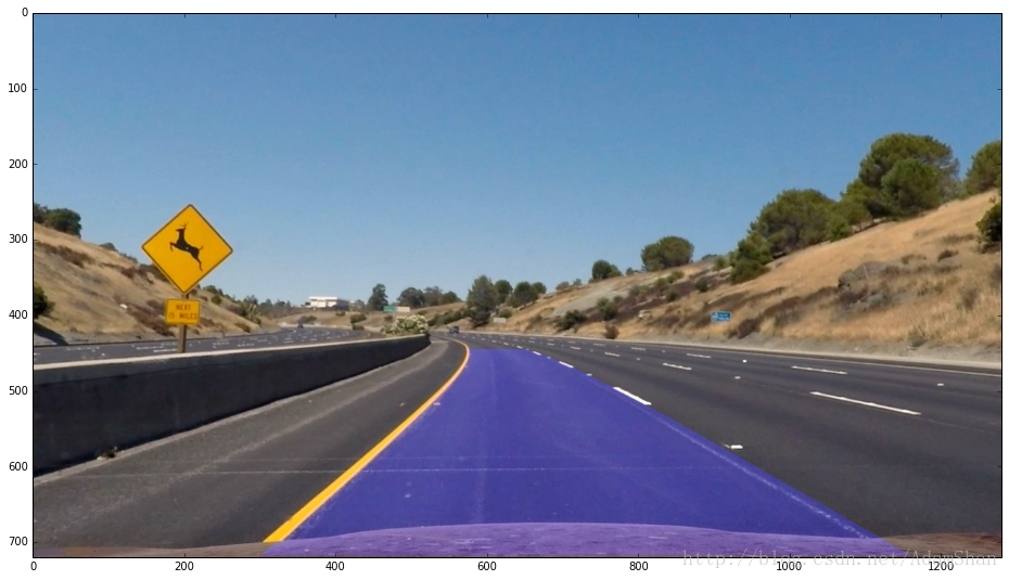
后记：在得到鸟瞰图的拟合曲线以后，我们是可以根据该曲线来计算车道的曲率的，同时如果知道车辆和相机的相对位置，还可以计算车辆距离左右车道线的距离，这就是目前基于视觉的车道偏离预警的实现方法之一，读者可以根据需要自行实现。

完整代码见：http://download.csdn.net/download/adamshan/10148446

AdamShan

关注

33
点赞
踩
220

收藏

觉得还不错? 一键收藏
打赏
23
评论
无人驾驶汽车系统入门（七）——基于传统计算机视觉的车道线检测(2)

无人驾驶汽车系统入门（七）——基于传统计算机视觉的车道线检测(2)原创不易，转载请注明来源：http://blog.csdn.net/adamshan/article/details/78733302接上文，在获得ROI（透视变换）以后，我们对得到的“鸟瞰图”应用色彩阈值化和梯度阈值化，以得到鸟瞰图中“可能为”车道线的像素然后再使用滑动窗口来确定车道线的多项式系数，下面我们来具体讨论这两个步骤。边缘
复制链接

扫一扫