基于模型预测控制(MPC)的最优竞赛（Matlab代码实现）

 💥💥💞💞欢迎来到本博客❤️❤️💥💥

🏆博主优势：🌞🌞🌞博客内容尽量做到思维缜密，逻辑清晰，为了方便读者。

⛳️座右铭：行百里者，半于九十。

📋📋📋本文目录如下：🎁🎁🎁

目录

💥1 概述

📚2 运行结果

🎉3 参考文献

🌈4 Matlab代码实现

---

💥1 概述

• 基于模型预测控制(MPC)的最优竞赛是一种优化问题，旨在通过控制系统的动态模型来最小化某个性能指标。在竞赛中，这个性能指标通常是比赛时间或者比赛得分。MPC是一种基于模型的控制方法，它使用系统的动态模型来预测未来的状态，并根据预测结果来生成最优的控制策略。

  在最优竞赛中，MPC可以用来生成最优的控制策略，以最小化比赛时间或得分。MPC的基本思想是在每个时间步骤上，使用系统的动态模型来预测未来的状态，并根据预测结果来生成最优的控制策略。这个控制策略可以是连续的，也可以是离散的，具体取决于竞赛的要求。

  MPC的优点是可以考虑到系统的动态特性和约束条件，从而生成最优的控制策略。此外，MPC还可以处理非线性系统和多变量系统，因此在竞赛中具有广泛的应用前景。

  总之，基于模型预测控制(MPC)的最优竞赛是一种优化问题，旨在通过控制系统的动态模型来最小化某个性能指标。MPC可以用来生成最优的控制策略，以最小化比赛时间或得分。MPC的优点是可以考虑到系统的动态特性和约束条件，因此在竞赛中具有广泛的应用前景。

本代码利用模型预测控制，使汽车选择转向命令，使其在模拟赛道上以最佳方式比赛。

​操作流程：

首先，转到并运行，添加到 MATLAB 路径:/utilsprecompute_grid.m/utils

然后回到主文件夹，现在您可以选择运行三个解决方案中的任何一个：

• 执行 MPC 的最简单解决方案，生成有效但次优轨迹：solution_1_simple_grid_search.m
• 执行更复杂的解决方案，以更优化的方式解决 MPC，但速度非常慢：solution_2_recursive_search.m
• 使用 fmincon 执行以进行持续优化，从而获得最佳结果:solution_3_fmincon.m

所需工具箱:

• Matlab（2022b年开发，不确定向后兼容性），
• Matlab 优化工具箱版本 9.4.，
• 统计和机器学习工具箱版本 12.5。

📚2 运行结果

主函数部分代码：

% setup
clear; clc;
close all; drawnow;
​
% loading Kosinka Grid and making the variables global
load("precompute_grid.mat")
global x_min_here
; x_min_here = x_min; 
global
 y_min_here; y_min_here = y_min; 
global
 spacing_here; spacing_here = spacing; 
global
 x_size_here; x_size_here = x_size; 
global
 y_size_here; y_size_here = y_size;global distances_here; distances_here = distances; global progresses_here; progresses_here = progresses;
% real cone positions from the map
% innerConePosition = [6.49447171658257,41.7389113024907;8.49189149682204,41.8037451937836;10.4848751821667,4692264908853,-8.52739205631154;-32.9016624434539,-6.87420998418598;-34.1160057737752,-1.60803776182190;-34.3261608207142,0.237322459171913;-34.4624174228984,2.11880932640591;-34.5407037273032,4.03273612643633;-34.5779532171168,5.97700580252438;-34.5920061096721,7.95066706685753;-34.6203010935088,11.9628384547546;-34.6463516562825,13.9656473217268;-34.6751545298116,15.9616504117489;-34.7230350194217,19.9334733431980;-34.7332354577762,21.9093507078716;-34.7284338451120,23.8784778261844;-34.6466389854161,27.7320065787716547;4.31684977705784,47.6749328204622;8.29483356036796,47.8005083348189];% load outer cone x and y coordinates
% assume constant width of the track, calculate from the first cones
in_x = innerConePosition(:,1); in_y = innerConePosition(:,2);
out_x = outerConePosition(:,1); out_y = outerConePosition(:,2);
w = sqrt((in_x(1)-out_x(1))^2+(in_y(1)-out_y(1))^2);
% generating track
[test_path_x, test_path_y] = generate_track(innerConePosition, outerConePosition);
​
% constants hashmap, which is also made global
keySet = ["tau", "width", "steps", "horizons", "global_steps", "min_speed", "max_speed", "max_acceleration", "max_brake", "steer_change", "lateral_acceleration", "max_steer", "intervals"];
valueSet = [0.01   w        50         3         1500          1                100            12              12            pi/6               50                  pi/3           3];
global constant; constant = containers.Map(keySet, valueSet);
​
% best choices at given moment: turning angle, progress along the line, acceleration
best_omega = 0; best = 0; best_a = 0;
​
% storing the path we actually took by taking the first step
taken_x = zeros(constant("global_steps"), 1); taken_x(1) = (in_x(1)+out_x(1))/2;
taken_y = zeros(constant("global_steps"), 1); taken_y(1) = (in_y(1)+out_y(1))/2;
taken_omega = zeros(constant("global_steps"), 1); taken_omega(1) = 0; % best omega to take
taken_theta = zeros(constant("global_steps"), 1); taken_theta(1) = 0; % best theta
taken_velocity = zeros(constant("global_steps"), 1); taken_velocity(1) = 1; % setting start velocity
taken_acceleration = zeros(constant("global_steps"), 1); taken_acceleration(1) = 0.1;
taken_best = zeros(constant("global_steps"), 1); taken_best(1) = 0; % best progress along the line
​
% bool to plot or not
plot_meanwhile = 1;
% plot the track to watch the car on
if plot_meanwhile == 1
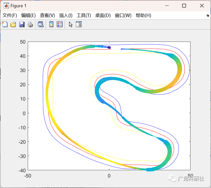
    figure; plot(test_path_x, test_path_y, 're', 'MarkerSize',5);
    hold on; plot(innerConePosition(:,1),innerConePosition(:,2),'ye','MarkerSize',5)
    hold on; plot(outerConePosition(:,1),outerConePosition(:,2),'bl','MarkerSize',5)
    hold on
end
​
% main loop
for a = 2:constant("global_steps")
    % update the current state
    current_velocity = taken_velocity(a-1); current_theta = taken_theta(a-1);
    current_x = taken_x(a-1); current_y = taken_y(a-1);
    current_omega = taken_omega(a-1); current_acceleration = taken_acceleration(a-1); current_best = taken_best(a-1);
​
    % watch the plot as it is generated
    if plot_meanwhile == 1
        scatter(current_x, current_y, 30, current_velocity+1, 'filled'); % path the model took: color = speed, size = change in angle
        hold on;
        pause(0.001)
    end
    % find the best move
    [best_a, best_omega, best_progress] = best_step_recursive(current_velocity, current_x, current_y, current_theta, constant("horizons"), current_acceleration, current_omega, current_best, constant("intervals"));
    % check if any move is possible
    if best_progress == -1
        upper "CRASHED"; break;
    end
    % let the model move
    [path_x, path_y, path_theta, velocities] = unicycle_model_acceleration_fixed(current_velocity, best_a, best_omega, current_x, current_y, current_theta, 2, constant("tau"), constant("max_speed"), constant("min_speed"));
    % save variables to keep track of the model
    taken_x(a)
 = path_x(
2
); taken_y(a) = path_y(
2
);    taken_omega(a) = best_omega; taken_acceleration(a) = best_a; taken_best(a) = best_progress;
    taken_theta(a) = path_theta(2); taken_velocity(a) = velocities(2);
end
​
% plotting all the curves at the end
figure; plot(test_path_x, test_path_y, 're', 'MarkerSize',5); % reference path to follow
hold on; plot(innerConePosition(:,1),innerConePosition(:,2),'ye','MarkerSize',5) % boundaries
hold on; plot(outerConePosition(:,1),outerConePosition(:,2),'bl','MarkerSize',5)
hold on; scatter(taken_x, taken_y, 30, taken_velocity+1, 'filled'); % path the model took: color = speed, size = change in angle
​
function [best_acceleration, best_omega, best_progress] = best_step_recursive(current_velocity, current_x, current_y, current_theta, horizons, last_acceleration, last_omega, last_progress, intervals)
    if horizons == 0 % recursion base case, return the last given variables
        best_acceleration = last_acceleration; best_omega = last_omega; best_progress = last_progress; return;
    end
    scored_scores = zeros(intervals, intervals); % keeping track of best scores
    global constant
    accelerations = linspace(-constant("max_brake"), constant("max_acceleration"), constant("intervals")); % generating accelerations
    for acceleration_index = 1:constant("intervals") % pick acceleration between limits and by braking and speeding up
        acceleration = accelerations(acceleration_index);
        max_velocity = max(current_velocity + acceleration*constant("tau")*constant("steps"), current_velocity); % maximum velocity on the next horizon
        omegas = linspace(max([-round(constant("lateral_acceleration")/max_velocity), -constant("max_steer"), last_omega - constant("steer_change")]), min([round(constant("lateral_acceleration")/max_velocity), last_omega + constant("steer_change"), constant("max_steer")]), constant("intervals")); % figure out viable angles
        for omega_index = 1:constant("intervals") % try angles
            omega = omegas(omega_index);
            % predict model movement 
            [path_x, path_y, path_theta, path_velocities] = unicycle_model_acceleration_fixed(current_velocity, acceleration, omega, current_x, current_y, current_theta, constant("steps"), constant("tau"), constant("max_speed"), constant("min_speed"));
            % check if path is valid by making x and y into indices on the grid
            global x_min_here; global y_min_here; global spacing_here; global x_size_here; global y_size_here;
            indices_x = floor((path_x-x_min_here)/x_size_here*spacing_here); indices_y = floor((path_y-y_min_here)/y_size_here*spacing_here);
            % take the maximum distance on the grid if all distances on the path are in the grid
            if max(indices_x) > spacing_here || min(indices_x) < 1 || max(indices_y) > spacing_here || min(indices_y) < 1
                continue
            end
            % find the maximum distance on the path
            global distances_here
; max_distance = max(distances_here(sub2ind([spacing_here, spacing_here],indices_x,indices_y)));            % if path within the lines, find the progress
            if max_distance < constant("width")/2
                global progresses_here; final_progress = progresses_here(indices_x(end), indices_y(end)); % find the maximum progress
                final_x = path_x(end); final_y = path_y(end);
                final_velocity = path_velocities(end); final_theta = path_theta(end);
                % make recursive call
                [~, ~, best_progress_now] = best_step_recursive(final_velocity, final_x, final_y, final_theta, horizons - 1, acceleration, omega, final_progress, intervals);
                scored_scores(acceleration_index, omega_index) = best_progress_now; % keep track of recursive progress
            end
        end
    end
    % if we did not get any valid action
    if scored_scores == zeros(intervals, intervals)
        best_acceleration = last_acceleration;
        best_omega = last_omega;
        best_progress = -1;
        return;
    end
    % pass back the maximal values from the recursive calls
    [max_progress, max_indices] = max(scored_scores(:));
    [max_x, max_y] = ind2sub(size(scored_scores), max_indices);
    best_acceleration = accelerations(max_x);
    best_omega = omegas(max_y);
    best_progress = max_progress;
end

🎉3 参考文献

[1]廖兴华. 基于MPC的FSAC赛车横向控制策略研究[D].西华大学,2020.​

部分理论引用网络文献，若有侵权联系博主删除。

🌈4 Matlab代码实现