基于模型预测(MPC)的四轮转向车辆轨迹规划（Matlab代码实现）

    目录

💥1 概述

📚2 运行结果

🎉3 参考文献

👨‍💻4 Matlab代码

💥1 概述

在轨迹跟踪应用领域，通常 MPC 建模可根据机器人的控制方式选择基于运动学运动状态方程建模或者基于动力学运动状态方程建模。前者是根据车辆转向的几何学角度关系和速度位置关系来建立描述车辆的运动的预测模型，一般只适用于低速运动场景；后者是对被控对象进行综合受力分析，从受力平衡的角度建模，一般应用在高速运动场景，如汽车无人驾驶。

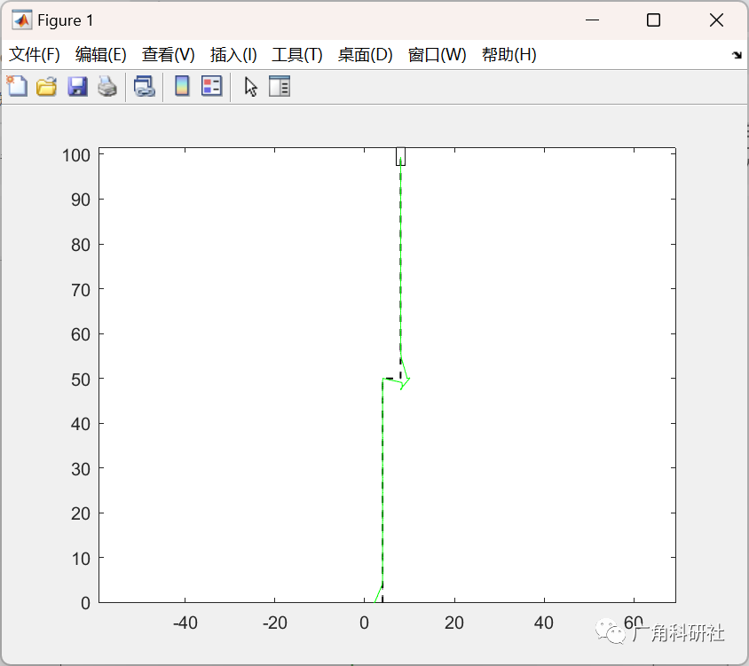
📚2 运行结果

主函数部分代码：

addpath(genpath('YALMIP-master'));
clear; close all;clc;
​
% constraints that is representing a car or a thiner road 
% final state with a higher weight to track the fianl state reference
​
%% Parameters definition
%
 model parametersparams.a_acc                = 1;                 % acceleration limit
params.a_dec                = 2;                   % decelerationlimit
params.delta_max            = 0.4;                 % maximum steering angle 
params.beta_max             = pi;                  % crabbing slip angle limit
params.beta_dot_max         = (pi/180)*(100);      % crabbing slip angle rate limit
params.l_f                  = 2;                   % distance between center of gravity and front axle
params.l_r                  = 2;                   % distance between center of gravity and rear axle
params.vehicle_width        = 2;                   % vehicle width
params.Ts                   = 0.1;                 % sampling time (both of MPC and simulated vehicle)
params.nstates              = 4;                   % number of states
params.ninputs              = 3;                   % number of inputs
​
% environment parameters
params.road                 = 'DLC';
params.activate_obstacles   = 0; 
params.obstacle_centers     = [10 -2; 20  0; 30 -2; 40 6]; % x and y coordinate of the 4 obstacles
params.obstacle_size        = [2 6];                    % size of the obstacles
switch params.road
    case 'real'
        [X,Y,X_park,Y_park]                   = data_generate(params.road);
    case 'DLC'
        [X,Y,X2,Y2]                   = data_generate(params.road);
    otherwise
        [X,Y]                   = data_generate(params.road);
end
params.X                    = X;
params.Y                    = Y;
params.lane_semiwidth       = 4;                        % semi-width of the lane
params.track_end_x          = X(end);                   % Tracking end X coordinate of the planner
params.track_end_y          = Y(end);                   % Tracking end Y coordinate of the planner
params.xlim                 = max(X);                   % x limit in the plot
params.ylim                 = max(Y);                   % y limit in the plot
​
​
​
% simulation parameters in frenet coord
params.s0                   = 0;                           % initial s coordinate
params.y0                   = params.lane_semiwidth/2;     % initial y coordinate
params.theta0               = pi/2;                        % initial relative heading angle
params.v0                   = 5;                          % initial speed
params.theta_c0             = pi/2;                        % initial heading angle of the curve
params.N_max                = 1000;                        % maximum number of simulation steps
params.vn                   = params.v0/2;                 % average speed during braking
params.vs                   = 1;                           % Stopping speed during the last stop 
​
%%% in this case, theta = theta_m (angle of the velocity vector)- theta_c (angle of the tangent vector of the curve)
​
% simulation parameters in cartesian coord %%%%% change according to
%
 different roadparams.x_c0                 = X(1)-params.y0; %initial x coordinate
params.y_c0                 = 0;                            % initial y coordinate
​
​
% plotting parameters
params.window_size          = 10;                       % plot window size for the
%during simulation, centered at the
%current position (x,y) of the vehicle
​
params.plot_full            = 1;                        % 0 for plotting only the window size,
​
​
% 1 for plotting from 0 to track_end
%% Simulation environment
%
 initializationsref         = zeros(params.N_max,1);
z            = zeros(params.N_max,params.nstates);             % z(k,j) denotes state j at step k-1(s and y)
z_cart       = zeros(params.N_max,3);                          % x,y coordinate in cartesian system and the heading angle
theta_c      = zeros(params.N_max,1);                          % initial value of theta_c
u            = zeros(params.N_max,params.ninputs);             % z(k,j) denotes input j at step k-1
z(1,:)       = [params.s0,params.y0,params.theta0,params.v0];  % definition of the intial state
z_cart(1,:)  = [params.x_c0,params.y_c0,params.theta0];
%theta_c(1)   = pi/2;    %%%%%% This value is changable according to different roads
comp_times   = zeros(params.N_max);                            % total computation time each sample
solve_times  = zeros(params.N_max);                            % optimization solver time each sample
i = 0;
N = 10;                                                 %predicted horizon length
m = params.N_max;
% formulating the reference of the system
switch params.road
    case 'real'
        path1 = [X;Y]';
        path2 = [X_park;Y_park]'
;        [S1, ~, ~, ~, ~] = getPathProperties(path1);
        num        = S1(end)/(params.v0*params.Ts);
        n_step1    = round(num);
        [S2, ~, ~, ~, ~] = getPathProperties(path2);
        num        = S2(end)/(params.vn*params.Ts);
        n_step2    = round(num);
        n_steps    = n_step1+n_step2;
        vq1         = linspace(Y(1),Y(end),n_step1);    % this need to be the 'variable' of the path function
        centerX1    = interp1(Y,X,vq1,'pchip');      % initialize the centerline y coordinate
        centerY1    = vq1;
        path_new_1   = [centerX1;centerY1]';
        vq2         = linspace(X_park(1),X_park(end),n_step2);
        centerY2    = interp1(X_park,Y_park,vq2,'
pchip
');      % initialize the centerline y coordinate
        centerX2    = vq2;
        path_new_2   = [centerX2;centerY2]'
;        path_new     = [path_new_1;path_new_2];
        [S, dX, dY, theta_c, C_c] = getPathProperties(path_new);
        theta_c_ref    = zeros(n_steps+N,1);
        C_c_ref        = zeros(n_steps+N,1);
        v_ref          = zeros(n_steps+N,1);
        for ii = 1:length(theta_c_ref)
            if ii<n_steps
                theta_c_ref(ii) = theta_c(ii);
                C_c_ref(ii)     = C_c(ii);
            else
                theta_c_ref(ii) = theta_c(end);
                C_c_ref(ii)     = C_c(end);
            end
        end
​

🎉3 参考文献

​[1]张鑫,吴伊凡,崔永琪.基于改进MPC算法的四旋翼无人机轨迹跟踪控制[J].电子技术与软件工程,2023,No.245(03):148-153.

部分理论引用网络文献，若有侵权联系博主删除。