【ConvexOptimization】1.Convex sets and functions

Disclaimer: This is a study note of the Fall 2018 Convex Optimization course offered at CMU. The note is compiled to document key understandings of concepts, which I think greatly aids the memorization and recalling process. While the note will inevitably borrow from the official class notes, I will refrain from any direct copy and paste to avoid copyrights violations. All references will be properly marked. The language will be English so that it might be shared with a wider audience.

Convex Problems, Convex Sets and Convex Functions

1. Convex Problems

1.1 Defining a convex optimization problem

• A convex problem minizes some convex $f(x)$ over $x$ with $x$ subject to both inequality and equality constraints.
• The inequality constraints are $g_i(x)\le 0$ constraints where each $g_i$ is convex.
• The equality constraints are $h_j(x)=0$ where $h_i$ are all affine functions.

Note the natural domain for $x$ $D$ is usually unconstrained (like ${\mathbb{R}}^n$) and usually convex. The equality constrains define some affine plane $Ax=b$ which also yields a convex set. We can prove for convex $g$, $g(x)\le 0$ also defines a convex set. Intersection preserves convexity. So we can say a convex problem minimizes a convex function over some particular convex set.

Further note that the equality constraints can only contain affine mappings of $x$ . Convex mappings are not enough for the equality constraints. This is intuitive because while a pie is a convex set, hollowed circle isn’t a convex set.

1.2 Property: Any local minimizer is a global minimizer

Say $x$ is a local minimizer, meaning we can find a neighborhood of $x$ with distance $ϵ$ such that within this neighborhood $f(x)$ is the minimizer. Take any $y$. If $f(y)<f(x)$, then take a convex combination $z$ of $x$ and $y$ that falls in the described neighborhood. Then $f(z)\le tf(x)+(1-t)f(y)<f(x)$, which contradicts the fact that $x$ is the local minimizer.

2. Convex Sets

2.1 Definitions

2.1.1 Convex Set

A set where the convex combination of any two members still belongs to the set.

2.1.2 Convex Combination

A linear combination where coefficients are all non-negative and sum up to 1.

2.1.3 Convex Hull

The smallest convex set containing the given set $S$.

2.2 Examples

2.2.1 Affine spaces

{ x : A x = b } \{x: Ax = b \} {x:Ax=b} for given $A,b$.

When $A$ is a vector, the set { x : a T x = b } \{x:a^Tx =b \} {x:aTx=b} represents a hyperplane. A hyperplane is a $n-1$ dimensional linear surface. IMHO, It is termed “hyper” because the dimension is $n-1$, which is usually high.

An affine space is just a shifted linear space. It can also be understood as the intersection of many hyperplanes.

{ x : A x ≤ b } \{ x: Ax \leq b \} {x:Ax≤b} is a polyhedron(多面体). It’s the intersection of many half spaces { x : a T x ≤ b } \{ x: a^Tx \leq b \} {x:aTx≤b}. The term “half space” truly reveals the nature of a hyperplan.

2.2.2 Simplex

A simplex is the convex hull of a set of affinely independent points.

Affine independence: points { x 0 , x 1 , x 2 , . . . , x n } \{ x_0, x_1, x_2, ..., x_n\} {x0​,x1​,x2​,...,xn​} are affinely independent iff { x 1 − x 0 , x 2 − x 0 , . . . , x n − x 0 } \{ x_1 - x_0, x_2 - x_0, ..., x_n - x_0\} {x1​−x0​,x2​−x0​,...,xn​−x0​} are linearly independent. In other words, if the affine plane passing through all $n$ points is of dimension $n-1$ (a hyperplane), the points are affinely independent.

Take { e 1 , . . . , e n } \{e_1, ..., e_n \} {e1​,...,en​} the standard basis, its simplex is called the “proability simplex”.

2.2.3 Cones

Intuitively, cones should contains rays emitting from any existing points.

• Cone: $C$ is a cone iff $x\in C$ yields $tx\in C$ for all $t\ge 0$ .
• Convex cone: A convex cone further contains everything inside the boundaries. More precisely, if $x_1$, $x_2$ are in the cone, then take any non-negative coefficients, $t_1{x}_1+t_2{x}_2\in C$
• Conic combination: any linear combination with non-negative coefficients. “Falls inside the boundary rays.”

Below are examples of convex cones:

• Norm Cone: { ( x , t ) : ∣ ∣ x ∣ ∣ ≤ t } \{ (x, t): ||x|| \leq t \} {(x,t):∣∣x∣∣≤t}. Note how this is different than a norm ball where the variable is $x$ alone.
• Normal Cone: for any given $C$, and $x\in C$, the normal cone is N C ( x ) = { g : g T ( y − x ) ≤ 0  for all y in C } \mathcal{N}_C(x) = \{g: g^T(y-x) \leq 0 \text{ for all y in C} \} NC​(x)={g:gT(y−x)≤0 for all y in C}.
  Geometrically, this means that $g$ is on different sides than any vector starting from $x$ and ending within the set $C$.
  Note by taking the normal cone of any point within any set, we get a convex cone.This is how we obtain convexity.
• PSD Cone: ${\mathbb{S}}_{+}^n$. the set of symmetric matrices that are Positive Semi Definite/ all eigenvalues nonnegative.

2.3 Important Properties

2.3.1 Separating Hyperplane Theorem

Theorem: two disjoint convex sets have a separating hyperplan between them.

Formally, if $C,D$ are nonempty convex sets such that $C\cap D=\varnothing$, then there exists $a,b$ such that
C ⊂ { x : a T x ≤ b } D ⊂ { x : a T x ≥ b } C \subset \{x: a^Tx \leq b\} \\ D \subset \{x: a^Tx \geq b \} C⊂{x:aTx≤b}D⊂{x:aTx≥b}

2.3.2 Supporting hyperplan theorem

Theorem: The boundary point of a convex set has a supporting hyperplane passing through it. A supporting hyperplane is the “tangent” hyperplane.

Formally, this means if $C$ is nonempty and convex, and for $x_0$ on its boundary, there exists an $a$ such that
C ⊂ { x : a T ( x − x 0 ) ≤ 0 } C \subset \{x: a^T(x - x_0) \leq 0 \} C⊂{x:aT(x−x0​)≤0}

The $a$ is the normal vector to the supporting hyperplane pointing outward.

2.4 Operations Preserving Convexity

2.4.1 Intersection

2.4.2 Scaling and Translation

Here the coefficients are limited to scalers

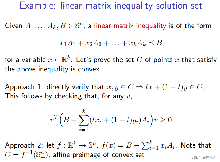
2.4.3 Affine image and preimage

Here the coefficients can be matrices.

The example below is quoted from lecture 2 note and quite illustrative.

2.4.4 Linear fractional images and preimages

$$f(x)=\frac{Ax+b}{c^{T}x+d}$$ where $c^{T}x+d>0$.

3. Convex Function

3.1 Definition

3.1.1 Convexity

A convex funciton is a function where for any two points in the domain, the secant line joining their functions values is always above or equal to the function.

3.1.2 Strict Convexity

…, the function is strictly below the line segments. Strict convexity means more curvature than the linear function .

3.1.3 Strongly Convex

with paramter $m>0$__: $f(x)-\frac{m||x|{|}^2}{2}$ is still convex. At least as curved as a quadratic .

3.2 Examples of Convex Functions

• Univariate function: exponentials are always convex; power functions when the power is greater than 1, and concave for power between 0 and 1; log is concave
• affine functions $a^{T}x+b$ are both convex and concave
• quadratic fucntions $x^{T}Qx+b^{T}x+c$ are convex provided $Q$ PSD
• least squared norms $||y-Ax|{|}^2$
• Norms. (Norms need to satisfy positivity, homogeneity(scaled norm = norm scaled), triangle inquality)
  The most common $l_p$ norms are $1,2,\infty$. $l_1$ is the sum of absolute values, and induces sparsity; $l_{\infty }$ is the max of magnitude of entries. Note$l_0$ (the number of non-zero entries) doesn’t satisfy homogenity so it’s not a norm.

3.3 Key properties

3.3.1 Epigraph characterization

A function being convex $⟺$ its epigraph (the area above or equal to the convex) is convex.

3.3.2 Convex sublevel sets

For any $t\in \mathbb{R}$, { x ∈ d o m ( f ) : f ( x ) ≤ t } \{x \in dom(f): f(x) \leq t \} {x∈dom(f):f(x)≤t} is convex.

3.3.3 First-order characterization of optimality

Given $f$ differentiable. For a minimizer $x$, take any $y$ satisfying the constraints, we have
$$\nabla f^T(y-x)\ge 0$$

This is saying the directional derivative is always non-negative starting from the minimizer. Directional derivatives only exist when gradients exist, and gradients are comprised of the function’s derivatives along the standard basis. In 1D, the gradient is 1D, and only 2 directions exist($y-x$ is either positive or negative). The above first order condition is equivalent to the derivative being both greater than or equal to zero.

3.3.4 First order characterization of convexity

$f$ convex $⟺$$f(y)-f(x)\ge \nabla f(x{)}^T(y-x)$

In words, the tangent line estimate always underestimates the change in function value.

3.3.5 Second-order characterization of convexity

The Hessian is positive semidefinite.

Note strict convexity doesn’t imply the Hessian is strictly positive definite.

3.3.6 Jensen’s inequality

The convex combination of { f ( x i ) } \{ f(x_i) \} {f(xi​)} is greater than the $f$ of the convex combination of $x_i$.

In probability theory this is $$\mathbb{E}(f(X))\ge f(\mathbb{E}(X))$$

3.3.7 Log-sum-exp function

$$g(x)=log({\Sigma }_{i=1}^k{e}^{a_i^{T}x+b_i})$$ smoothly approximates the maximum of $a_i^{T}x+b_i$, so it’s called the softmax.

3.4 Operations Preserving Convexity

3.4.1 Non-negative linear combinations

Note taking the negative would change the convexity.

3.4.2 Pointwise maximization

Over a set of functions.

3.4.3 Partial minimization.

This allows the transformation of the original problem. The hinge loss form of SVM is an example.