


Apollo的的规划算法基于Frenet坐标系,因此道路中心线的平滑性控制着车辆是否左右频繁晃动,而高精地图的道路中心线往往不够平滑。
离散点平滑法,包括
1,FEM_POS_DEVIATION_SMOOTHING有限元位置差异
2,COS_THETA_SMOOTHING余弦)
3,QpSplineReferenceLineSmoother(三次样条插值法)
4,SpiralReferenceLineSmoother(螺旋曲线法)
本文只讲解FEM_POS_DEVIATION_SMOOTHING有限元位置差异的方法。
一,为什么需要重新生成参考线
导航路径存在的问题:1,导航路径过长;2,不平滑
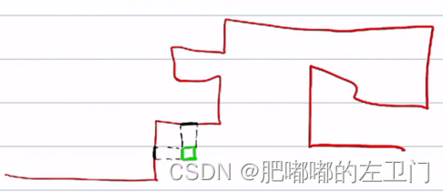
导致的结果:
1,不利于主车以及障碍物寻找投影点,甚至出现多个投影点。
2,原本的导航路径不平滑,车辆无法直接进行轨迹跟踪。
解决方案:根据导航路径,生成参考线。
二,生成参考线的具体步骤与方法
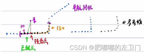
1,找到匹配点以及投影点
2,以匹配点或者投影点为原点,往后取30个点,往前取150个点。对这180个点进行平滑处理,生成符合要求的参考线,作为该规划周期内的参考线,并以此参考线为Frenet坐标系。
三,参考线平滑方法:QP
方法步骤:
1,设计Cost:平滑程度,与原路径的偏离程度,路径点距离分布的均匀程度。
2,整理Cost目标函数,使其符合QP的表达形式。
3,考虑约束条件,并整理为QP的约束表达式形式。
4,运用合适的QP求解器进行求解,获取优化后的结果。
四,设计Cost:平滑程度,与原路径的偏离程度,路径点距离分布的均匀程度(长度代价)
1,平滑程度

衡量指标:。其值越小, 路径越平滑。
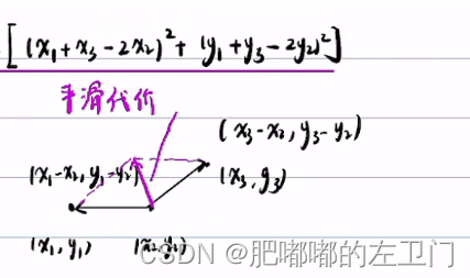
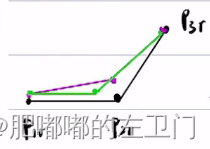
2,与原路径的偏离程度
如上图所示,平滑前的点记为,平滑后的点记为
。
虽然路径平滑了,但与原路径距离偏差太大,不符合要求。
衡量指标:
3,路径点距离分布的均匀程度(长度代价)
衡量指标:。其值越小,分布越均匀。
五,实例讲解
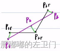
1,以3个点为例求解目标函数
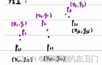
如上图所示,已知变量:原路径点为:,未知变量:优化后的路径点为:
,求优化后的路径点坐标。
2,二次规划的一般形式
3,n个点的代价函数求解(重点):
平滑性代价:
其中:
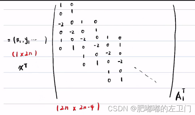
令
则
均匀性代价(长度代价):
其中,
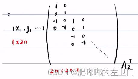
令
则
与原路径的距离偏差代价:
由于是常数,对目标函数的变化没有影响,故可以删除,以简化表达。
令,
则:
综述所述:
一般情况下,平滑的权重系数远远大于其他2项的权重系数
二次规划的标准形式为:
则
求解约束条件:
至此,参考线平滑问题转化为二次规划的标准形式,采用成熟的求解器求解即可获得,从而实现导航轨迹的平滑,获得符合要求的参考线轨迹点。
import osqp
import numpy as np
import matplotlib.pyplot as plt
from scipy import sparse
#计算kappa用来评价曲线
def calcKappa(x_array,y_array):
s_array = []
k_array = []
if(len(x_array) != len(y_array)):
return(s_array , k_array)
length = len(x_array)
temp_s = 0.0
s_array.append(temp_s)
for i in range(1 , length):
temp_s += np.sqrt(np.square(y_array[i] - y_array[i - 1]) + np.square(x_array[i] - x_array[i - 1]))
s_array.append(temp_s)
xds,yds,xdds,ydds = [],[],[],[]
for i in range(length):
if i == 0:
xds.append((x_array[i + 1] - x_array[i]) / (s_array[i + 1] - s_array[i]))
yds.append((y_array[i + 1] - y_array[i]) / (s_array[i + 1] - s_array[i]))
elif i == length - 1:
xds.append((x_array[i] - x_array[i-1]) / (s_array[i] - s_array[i-1]))
yds.append((y_array[i] - y_array[i-1]) / (s_array[i] - s_array[i-1]))
else:
xds.append((x_array[i+1] - x_array[i-1]) / (s_array[i+1] - s_array[i-1]))
yds.append((y_array[i+1] - y_array[i-1]) / (s_array[i+1] - s_array[i-1]))
for i in range(length):
if i == 0:
xdds.append((xds[i + 1] - xds[i]) / (s_array[i + 1] - s_array[i]))
ydds.append((yds[i + 1] - yds[i]) / (s_array[i + 1] - s_array[i]))
elif i == length - 1:
xdds.append((xds[i] - xds[i-1]) / (s_array[i] - s_array[i-1]))
ydds.append((yds[i] - yds[i-1]) / (s_array[i] - s_array[i-1]))
else:
xdds.append((xds[i+1] - xds[i-1]) / (s_array[i+1] - s_array[i-1]))
ydds.append((yds[i+1] - yds[i-1]) / (s_array[i+1] - s_array[i-1]))
for i in range(length):
k_array.append((xds[i] * ydds[i] - yds[i] * xdds[i]) / (np.sqrt(xds[i] * xds[i] + yds[i] * yds[i]) * (xds[i] * xds[i] + yds[i] * yds[i]) + 1e-6));
return(s_array,k_array)
def referenceline():
#add some data for test
x_array = [0.5,1.0,2.0,3.0,4.0,
5.0,6.0,7.0,8.0,9.0,
10.0,11.0,12.0,13.0,14.0,
15.0,16.0,17.0,18.0,19.0]
y_array = [0.1,0.3,0.2,0.4,0.3,
-0.2,-0.1,0,0.5,0,
0.1,0.3,0.2,0.4,0.3,
-0.2,-0.1,0,0.5,0]
length = len(x_array)
#weight , from config
weight_fem_pos_deviation_ = 1e10 #cost1 - x
weight_path_length = 1 #cost2 - y
weight_ref_deviation = 1 #cost3 - z
P = np.zeros((length,length))
#set P matrix,from calculateKernel
#add cost1
P[0,0] = 1 * weight_fem_pos_deviation_
P[0,1] = -2 * weight_fem_pos_deviation_
P[1,1] = 5 * weight_fem_pos_deviation_
P[length - 1 , length - 1] = 1 * weight_fem_pos_deviation_
P[length - 2 , length - 1] = -2 * weight_fem_pos_deviation_
P[length - 2 , length - 2] = 5 * weight_fem_pos_deviation_
for i in range(2 , length - 2):
P[i , i] = 6 * weight_fem_pos_deviation_
for i in range(2 , length - 1):
P[i - 1, i] = -4 * weight_fem_pos_deviation_
for i in range(2 , length):
P[i - 2, i] = 1 * weight_fem_pos_deviation_
with np.printoptions(precision=0):
print(P)
P = P / weight_fem_pos_deviation_
P = sparse.csc_matrix(P)
#set q matrix , from calculateOffset
q = np.zeros(length)
#set Bound(upper/lower bound) matrix , add constraints for x
#from CalculateAffineConstraint
#In apollo , Bound is from road boundary,
#Config limit with (0.1,0.5) , Here I set a constant 0.2
bound = 0.2
A = np.zeros((length,length))
for i in range(length):
A[i, i] = 1
A = sparse.csc_matrix(A)
lx = np.array(x_array) - bound
ux = np.array(x_array) + bound
ly = np.array(y_array) - bound
uy = np.array(y_array) + bound
#solve
prob = osqp.OSQP()
prob.setup(P,q,A,lx,ux)
res = prob.solve()
opt_x = res.x
prob.update(l=ly, u=uy)
res = prob.solve()
opt_y = res.x
#plot x - y , opt_x - opt_y , lb - ub
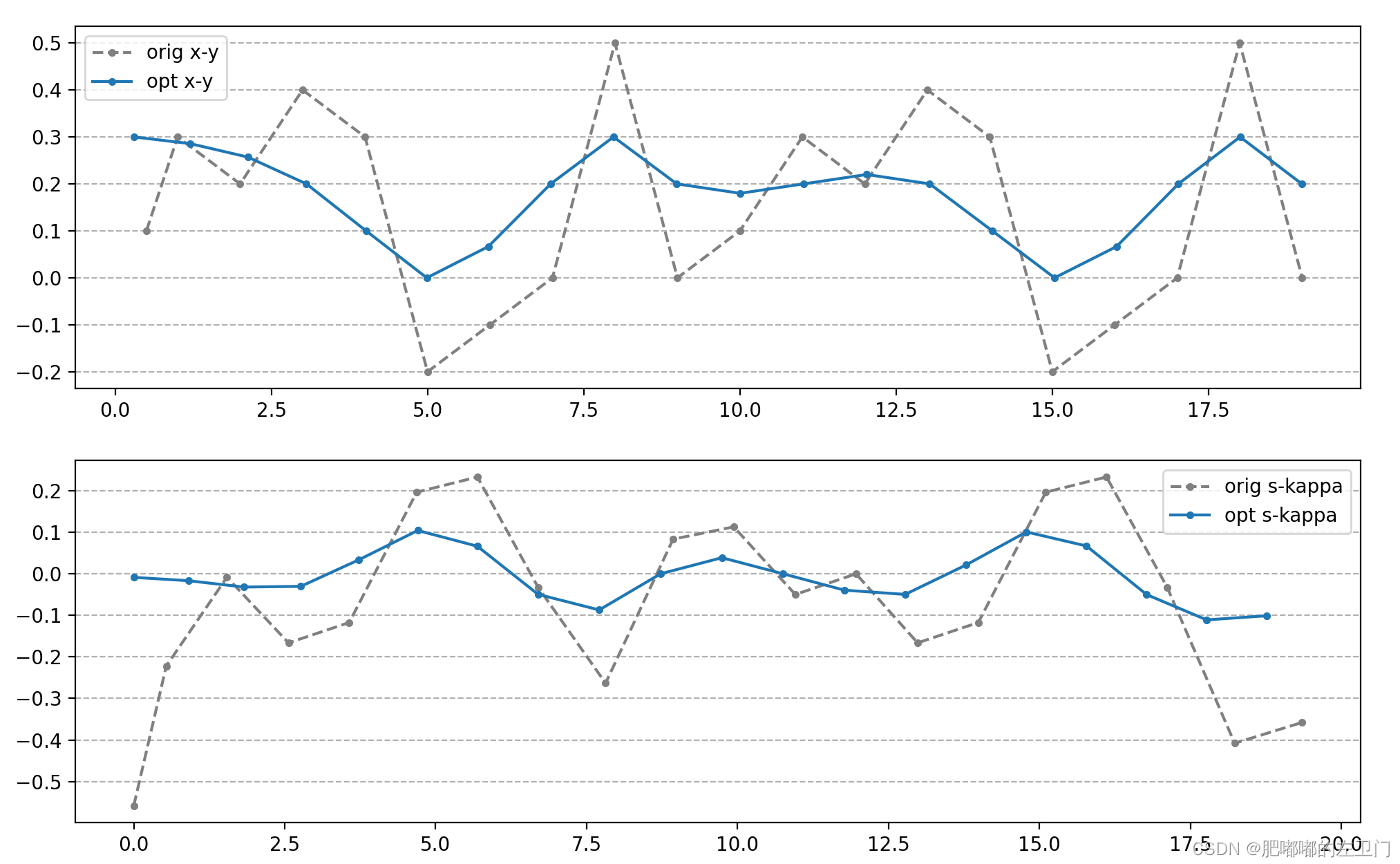
fig1 = plt.figure(dpi = 100 , figsize=(12, 8))
ax1_1 = fig1.add_subplot(2,1,1)
ax1_1.plot(x_array,y_array , ".--", color = "grey", label="orig x-y")
ax1_1.plot(opt_x, opt_y,".-",label = "opt x-y")
# ax1_1.plot(x_array,ly,".--r",label = "bound")
# ax1_1.plot(x_array,uy,".--r")
ax1_1.legend()
ax1_1.grid(axis="y",ls='--')
#plot kappa
ax1_2 = fig1.add_subplot(2,1,2)
s_orig,k_orig = calcKappa(x_array,y_array)
s_opt ,k_opt = calcKappa(opt_x,opt_y)
ax1_2.plot(s_orig , k_orig , ".--", color = "grey", label="orig s-kappa")
ax1_2.plot(s_opt,k_opt,".-",label="opt s-kappa")
ax1_2.legend()
ax1_2.grid(axis="y",ls='--')
plt.show()
if __name__ == '__main__':
referenceline()
平滑前后的坐标和曲率对比:


 1966
1966


 被折叠的 条评论
为什么被折叠?
被折叠的 条评论
为什么被折叠?
 到【灌水乐园】发言


