Vision Transformer：ViT网络结构

前言

• 由于本人水平有限，难免出现错漏，敬请批评改正。
• 更多精彩内容，可点击进入人工智能知识点专栏、Python日常小操作专栏、OpenCV-Python小应用专栏、YOLO系列专栏、自然语言处理专栏或我的个人主页查看
• 基于DETR的人脸伪装检测
• YOLOv7训练自己的数据集（口罩检测）
• YOLOv8训练自己的数据集（足球检测）
• YOLOv5：TensorRT加速YOLOv5模型推理
• YOLOv5：IoU、GIoU、DIoU、CIoU、EIoU
• 玩转Jetson Nano（五）：TensorRT加速YOLOv5目标检测
• YOLOv5：添加SE、CBAM、CoordAtt、ECA注意力机制
• YOLOv5：yolov5s.yaml配置文件解读、增加小目标检测层
• Python将COCO格式实例分割数据集转换为YOLO格式实例分割数据集
• YOLOv5：使用7.0版本训练自己的实例分割模型（车辆、行人、路标、车道线等实例分割）
• 使用Kaggle GPU资源免费体验Stable Diffusion开源项目

相关介绍

• 论文地址：https://arxiv.org/abs/2010.11929
• 官方源代码地址：https://github.com/google-research/vision_transformer
• 有兴趣可查阅论文和官方源代码地址。

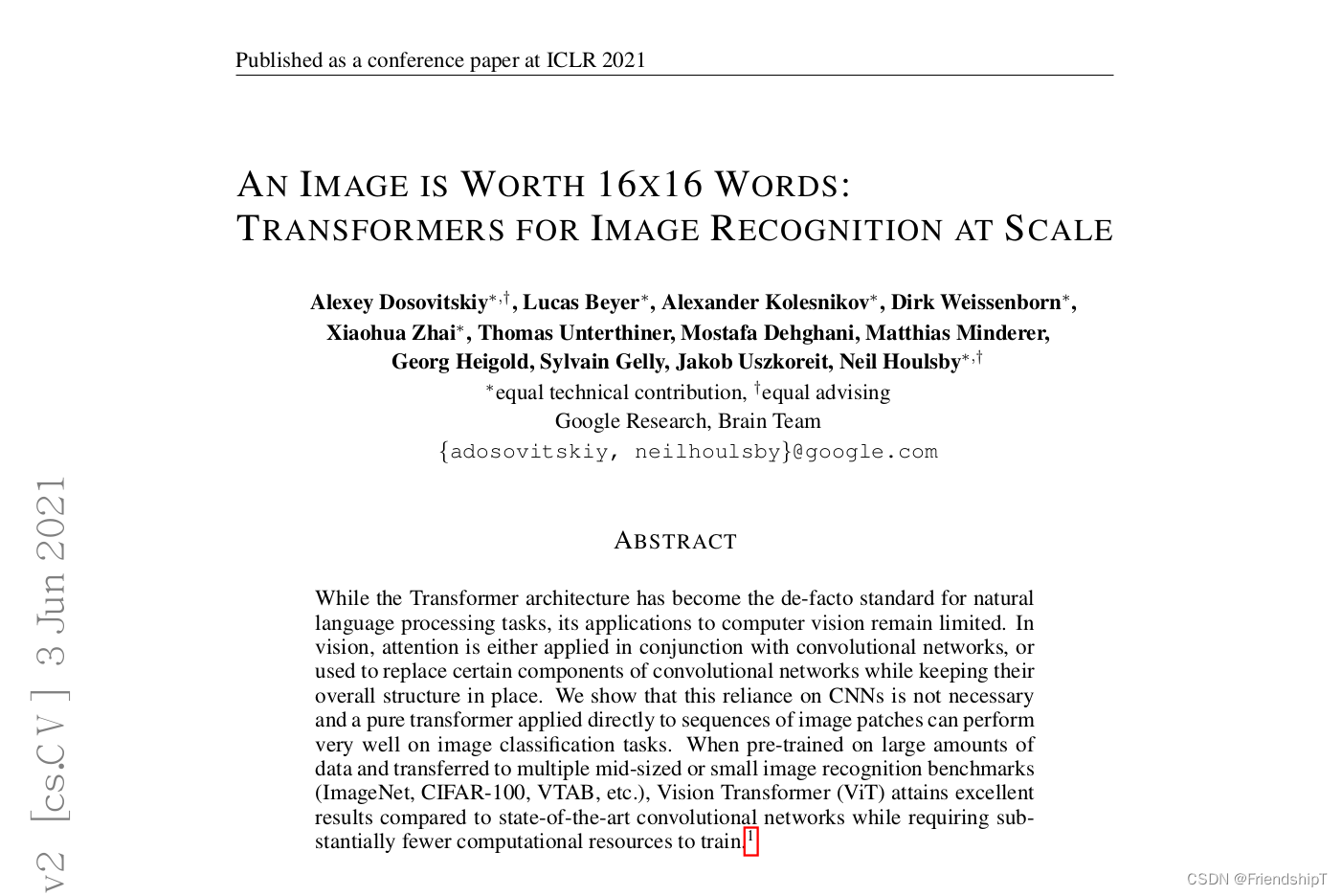
Vision Transformer（ViT）是谷歌在2020年提出的一种革命性的图像处理模型，它首次成功地将Transformer架构应用于计算机视觉领域，尤其是图像分类任务。之前，卷积神经网络（CNN）在视觉任务上一直占据主导地位，而ViT模型的成功表明Transformer架构也可以高效处理视觉信号。

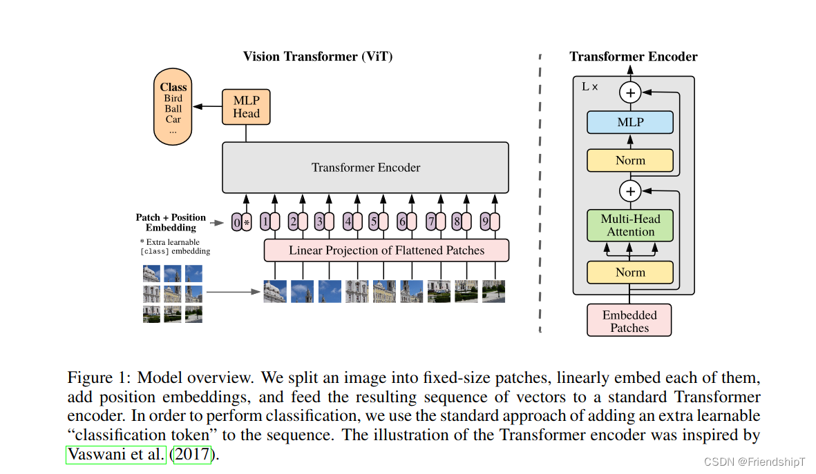
ViT模型的基本原理：

1. 输入预处理：
   ViT首先将输入图像分成固定大小的 patches（通常是16x16像素的小块），并将每个patch视为一个单词。接着，每个patch通过一个线性嵌入层转换成一个高维向量，类似于词嵌入在NLP中的作用。

2. 位置编码：
   类似于NLP中的Transformer，ViT也需要位置编码以保留图像块的空间信息，因为Transformer自身并不具备顺序信息。这通常通过向每个patch嵌入添加一个位置编码向量来实现。

3. Transformer Encoder堆叠：
   获得的patch嵌入序列随后馈送到一系列的Transformer Encoder层中。每个Encoder层包含一个多头自注意力模块（Multi-Head Self-Attention）和一个前馈神经网络（FFN）。这些层允许模型捕获全局依赖关系，而不是局限于局部感受野。

4. 分类头部：
   与BERT等NLP模型类似，ViT模型的最后一层输出被连接到一个分类头部。对于图像分类任务，这通常是一个线性层，其输出维度对应于类别数量。

5. 训练与评估：
   ViT模型通常在大规模图像数据集上训练，如ImageNet，并在验证集上进行评估，结果显示即使在有限的数据集上训练，随着模型规模的增大，ViT也能取得非常优秀的性能。

ViT的特点与优势：

• 全局建模能力：由于自注意力机制，ViT可以同时考虑图像的所有部分，有利于捕捉全局上下文信息。
• 并行化处理：Transformer的自注意力机制天然支持并行计算，有助于提高训练效率。
• 可扩展性：随着模型容量的增加，ViT的表现通常能持续提升，尤其在大模型和大数据集上表现出色。
• 统一架构：ViT将视觉和语言的处理方式统一到Transformer架构下，促进了跨模态学习的发展。

ViT的缺点：

尽管Vision Transformer (ViT)在许多方面展现出了强大的潜力和优越性，但它也存在一些不足之处：

1. 大量数据需求：
   ViT在较小的数据集上容易过拟合，尤其是在从头开始训练时。与卷积神经网络相比，ViT通常需要更大的训练数据集才能达到最佳性能。为了解决这个问题，后续的研究提出了诸如DeiT（Data-efficient Image Transformers）等技术，利用知识蒸馏等手段来降低对大规模数据集的依赖。

2. 计算资源消耗：
   ViT模型的训练和推理通常需要更多的计算资源，包括内存和GPU时间。自注意力机制涉及全图谱的计算，对于长序列或者高分辨率的图像，这种计算成本可能会变得相当高昂。

3. 缺乏局部特征提取：
   ViT直接将图像划分为patches，虽然能够捕获全局信息，但在处理图像局部细节和纹理时可能不如卷积神经网络精细。为了解决这个问题，后来的变体如Swin Transformer引入了分层和局部窗口注意力机制。

4. 迁移学习与微调：
   初始阶段，ViT在下游任务上的迁移学习和微调可能不如经过长期优化的传统CNNs如ResNet方便。不过，随着预训练模型如ImageNet-21K和JFT-300M上训练的大规模ViT模型的发布，这一问题得到了一定程度的缓解。

5. 复杂度和速度：
   相较于轻量级的卷积神经网络，ViT在某些实时或边缘设备上的部署可能受限于其较高的计算复杂度和延迟。

尽管存在上述挑战，但随着研究的深入和硬件技术的进步，许多针对ViT的改进方案已经被提出并有效地解决了部分问题，使其在众多视觉任务中展现出越来越强的竞争力。

应用与拓展：

自从ViT提出以来，研究人员不断对其进行了各种改进和扩展，包括但不限于DeiT（Data-efficient Image Transformers）、Swin Transformer（引入了窗口注意力机制）、PVT（Pyramid Vision Transformer）等，使得Transformer架构在更多视觉任务，如目标检测、语义分割等上取得了很好的效果，并逐渐成为视觉模型设计的新范式。

网络结构

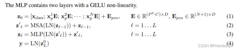
Embedding 层

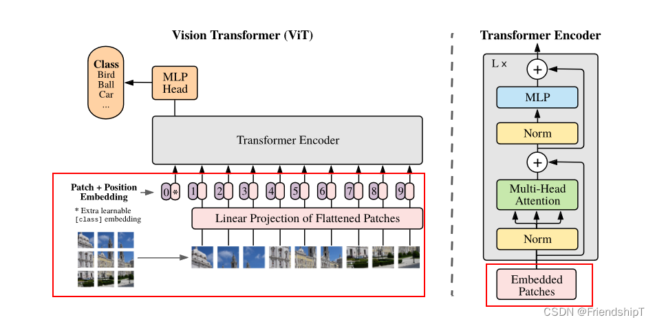
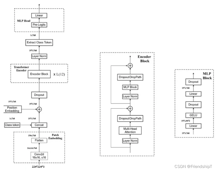
对于标准的 Transformer 模块，要求的输入是 token 向量的序列，即二维矩阵 [num_token, token_dim]。在具体的代码实现过程中呢，我们实际是通过一个卷积层来实现以 ViT-B/16 为例，使用卷积核大小为 16 × 16, stride 为 16，卷积核个数为 768 来实现的，即 [224,224,3] --> [14,14,768] --> [196, 768]。即一共 196 个token，每个 token 向量长度为 768。此外我们还需要加上一个类别的 token，为此我们实际上是初始化了一个可训练的参数 [1, 768]，将其与 token 序列进行拼接得到 Cat([1, 768], [196,768]) --> [197, 768]。然后再叠加上位置编码 Position Embedding: [197,768] --> [197, 768]。

class Embeddings(nn.Module):
    """Construct the embeddings from patch, position embeddings.
    """
    def __init__(self, config, img_size, in_channels=3):
        super(Embeddings, self).__init__()
        self.hybrid = None
        img_size = _pair(img_size)

        if config.patches.get("grid") is not None:
            grid_size = config.patches["grid"]
            patch_size = (img_size[0] // 16 // grid_size[0], img_size[1] // 16 // grid_size[1])
            n_patches = (img_size[0] // 16) * (img_size[1] // 16)
            self.hybrid = True
        else:
            patch_size = _pair(config.patches["size"])
            n_patches = (img_size[0] // patch_size[0]) * (img_size[1] // patch_size[1])
            self.hybrid = False

        if self.hybrid:
            self.hybrid_model = ResNetV2(block_units=config.resnet.num_layers,
                                         width_factor=config.resnet.width_factor)
            in_channels = self.hybrid_model.width * 16
        self.patch_embeddings = Conv2d(in_channels=in_channels,
                                       out_channels=config.hidden_size,
                                       kernel_size=patch_size,
                                       stride=patch_size)
        self.position_embeddings = nn.Parameter(torch.zeros(1, n_patches+1, config.hidden_size))
        self.cls_token = nn.Parameter(torch.zeros(1, 1, config.hidden_size))

        self.dropout = Dropout(config.transformer["dropout_rate"])

    def forward(self, x):
        # print(x.shape)
        B = x.shape[0]
        cls_tokens = self.cls_token.expand(B, -1, -1)
        # print(cls_tokens.shape)
        if self.hybrid:
            x = self.hybrid_model(x)
        x = self.patch_embeddings(x)#Conv2d: Conv2d(3, 768, kernel_size=(16, 16), stride=(16, 16))
        # print(x.shape)
        x = x.flatten(2)
        # print(x.shape)
        x = x.transpose(-1, -2)
        # print(x.shape)
        x = torch.cat((cls_tokens, x), dim=1)
        # print(x.shape)

        embeddings = x + self.position_embeddings
        # print(embeddings.shape)
        embeddings = self.dropout(embeddings)
        # print(embeddings.shape)
        return embeddings

Transformer Encoder 层

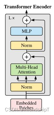
Transformer Encoder 就是将 Encoder Block 重复堆叠 L 次。我们来看看单个 Encoder Block。首先输入一个 Norm 层，这里的 Norm 指的是 Layer Normalization 层（有论文比较了 BN 在 transformer 中为什么不好，不如 LN ｜这里先 Norm 再 Multihead Attention 也是有论文研究的，原始的 Transformer 先 Attention 再 Norm，此外这个先 Norm 再操作和 DenseNet 的先 BN 再 Conv 异曲同工）。经过 LN 后经过 Multi-Head Attention，然后源码经过 Dropout 层，有些复现大神使用的是 DropPath 方法，根据以往的经验可能使用后者会更好一点。然后残差之后经过 LN，MLP Block，Dropout/DropPath 之后残差即可。

MLP Block 其实也很简单，就是一个全连接，GELU 激活函数，Dropout，全连接，Dropout。需要注意第一个全连接层的节点个数是输入向量长度的 4 倍，第二个全连接层会还原会原来的大小。

注意：在源码里，在 Transformer Encoder 前有个 Dropout 层，在之后有一个 Layer Norm 层。

class Block(nn.Module):
    def __init__(self, config, vis):
        super(Block, self).__init__()
        self.hidden_size = config.hidden_size
        self.attention_norm = LayerNorm(config.hidden_size, eps=1e-6)
        self.ffn_norm = LayerNorm(config.hidden_size, eps=1e-6)
        self.ffn = Mlp(config)
        self.attn = Attention(config, vis)

    def forward(self, x):
        # print(x.shape)
        h = x
        x = self.attention_norm(x)
        # print(x.shape)
        x, weights = self.attn(x)
        x = x + h
        # print(x.shape)

        h = x
        x = self.ffn_norm(x)
        # print(x.shape)
        x = self.ffn(x)
        # print(x.shape)
        x = x + h
        # print(x.shape)
        return x, weights

class Encoder(nn.Module):
    def __init__(self, config, vis):
        super(Encoder, self).__init__()
        self.vis = vis
        self.layer = nn.ModuleList()
        self.encoder_norm = LayerNorm(config.hidden_size, eps=1e-6)
        for _ in range(config.transformer["num_layers"]):
            layer = Block(config, vis)
            self.layer.append(copy.deepcopy(layer))

    def forward(self, hidden_states):
        # print(hidden_states.shape)
        attn_weights = []
        for layer_block in self.layer:
            hidden_states, weights = layer_block(hidden_states)
            if self.vis:
                attn_weights.append(weights)
        encoded = self.encoder_norm(hidden_states)
        return encoded, attn_weights


class Transformer(nn.Module):
    def __init__(self, config, img_size, vis):
        super(Transformer, self).__init__()
        self.embeddings = Embeddings(config, img_size=img_size)
        self.encoder = Encoder(config, vis)

    def forward(self, input_ids):
        embedding_output = self.embeddings(input_ids)
        encoded, attn_weights = self.encoder(embedding_output)
        return encoded, attn_weights

Multi-Head Attention 层

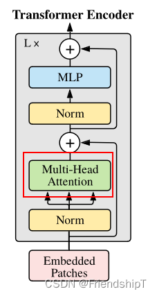
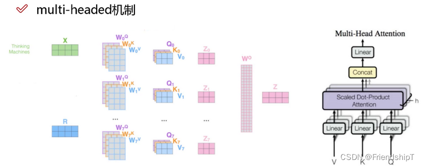
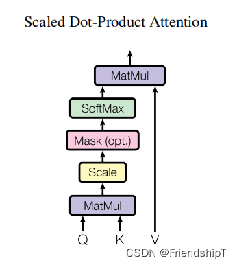
多头自注意力时，先将输入映射到q，k，v，如果只有一个头，qkv的维度都是197x768，如果有12个头（768/12=64），则qkv的维度是197x64，一共有12组qkv，最后再将12组qkv的输出拼接起来，输出维度是197x768，然后在过一层LN，维度依然是197x768

class Attention(nn.Module):
    def __init__(self, config, vis):
        super(Attention, self).__init__()
        self.vis = vis
        self.num_attention_heads = config.transformer["num_heads"]
        self.attention_head_size = int(config.hidden_size / self.num_attention_heads)
        self.all_head_size = self.num_attention_heads * self.attention_head_size

        self.query = Linear(config.hidden_size, self.all_head_size)
        self.key = Linear(config.hidden_size, self.all_head_size)
        self.value = Linear(config.hidden_size, self.all_head_size)

        self.out = Linear(config.hidden_size, config.hidden_size)
        self.attn_dropout = Dropout(config.transformer["attention_dropout_rate"])
        self.proj_dropout = Dropout(config.transformer["attention_dropout_rate"])

        self.softmax = Softmax(dim=-1)

    def transpose_for_scores(self, x):
        new_x_shape = x.size()[:-1] + (self.num_attention_heads, self.attention_head_size)
        # print(new_x_shape)
        x = x.view(*new_x_shape)
        # print(x.shape)
        # print(x.permute(0, 2, 1, 3).shape)
        return x.permute(0, 2, 1, 3)

    def forward(self, hidden_states):
        # print(hidden_states.shape)
        mixed_query_layer = self.query(hidden_states)#Linear(in_features=768, out_features=768, bias=True)
        # print(mixed_query_layer.shape)
        mixed_key_layer = self.key(hidden_states)
        # print(mixed_key_layer.shape)
        mixed_value_layer = self.value(hidden_states)
        # print(mixed_value_layer.shape)

        query_layer = self.transpose_for_scores(mixed_query_layer)
        # print(query_layer.shape)
        key_layer = self.transpose_for_scores(mixed_key_layer)
        # print(key_layer.shape)
        value_layer = self.transpose_for_scores(mixed_value_layer)
        # print(value_layer.shape)

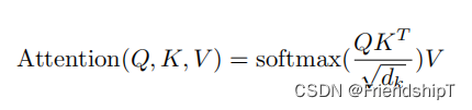
        attention_scores = torch.matmul(query_layer, key_layer.transpose(-1, -2))
        # print(attention_scores.shape)
        attention_scores = attention_scores / math.sqrt(self.attention_head_size)
        # print(attention_scores.shape)
        attention_probs = self.softmax(attention_scores)
        # print(attention_probs.shape)
        weights = attention_probs if self.vis else None
        attention_probs = self.attn_dropout(attention_probs)
        # print(attention_probs.shape)

        context_layer = torch.matmul(attention_probs, value_layer)
        # print(context_layer.shape)
        context_layer = context_layer.permute(0, 2, 1, 3).contiguous()
        # print(context_layer.shape)
        new_context_layer_shape = context_layer.size()[:-2] + (self.all_head_size,)
        context_layer = context_layer.view(*new_context_layer_shape)
        # print(context_layer.shape)
        attention_output = self.out(context_layer)
        # print(attention_output.shape)
        attention_output = self.proj_dropout(attention_output)
        # print(attention_output.shape)
        return attention_output, weights

MLP（Multilayer Perceptron） Head 层

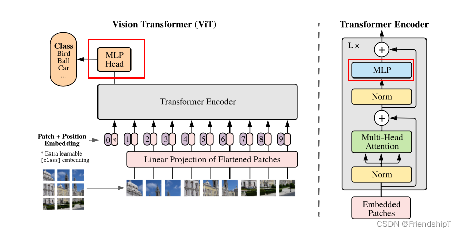
MLP（Multilayer Perceptron）多层感知机：将维度放大再缩小回去，197x768放大为197x3072，再缩小变为197x768

一个block之后维度依然和输入相同，都是197x768，因此可以堆叠多个block。最后会将特殊字符cls对应的输出，作为encoder的最终输出 ，后面接一个MLP进行图片分类。

class Mlp(nn.Module):
    def __init__(self, config):
        super(Mlp, self).__init__()
        self.fc1 = Linear(config.hidden_size, config.transformer["mlp_dim"])
        self.fc2 = Linear(config.transformer["mlp_dim"], config.hidden_size)
        self.act_fn = ACT2FN["gelu"]
        self.dropout = Dropout(config.transformer["dropout_rate"])

        self._init_weights()

    def _init_weights(self):
        nn.init.xavier_uniform_(self.fc1.weight)
        nn.init.xavier_uniform_(self.fc2.weight)
        nn.init.normal_(self.fc1.bias, std=1e-6)
        nn.init.normal_(self.fc2.bias, std=1e-6)

    def forward(self, x):
        x = self.fc1(x)
        x = self.act_fn(x)
        x = self.dropout(x)
        x = self.fc2(x)
        x = self.dropout(x)
        return x

参考

[1] Alexey Dosovitskiy, Lucas Beyer, Alexander Kolesnikov, Dirk Weissenborn, Xiaohua Zhai, Thomas Unterthiner, Mostafa Dehghani, Matthias Minderer, Georg Heigold, Sylvain Gelly, Jakob Uszkoreit, Neil Houlsby. An Image is Worth 16x16 Words: Transformers for Image Recognition at Scale. 2020
[2] ViT源代码地址. https://github.com/google-research/vision_transformer
[3] https://zhuanlan.zhihu.com/p/642007768
[4] https://zhuanlan.zhihu.com/p/445122996

• 由于本人水平有限，难免出现错漏，敬请批评改正。
• 更多精彩内容，可点击进入人工智能知识点专栏、Python日常小操作专栏、OpenCV-Python小应用专栏、YOLO系列专栏、自然语言处理专栏或我的个人主页查看
• 基于DETR的人脸伪装检测
• YOLOv7训练自己的数据集（口罩检测）
• YOLOv8训练自己的数据集（足球检测）
• YOLOv5：TensorRT加速YOLOv5模型推理
• YOLOv5：IoU、GIoU、DIoU、CIoU、EIoU
• 玩转Jetson Nano（五）：TensorRT加速YOLOv5目标检测
• YOLOv5：添加SE、CBAM、CoordAtt、ECA注意力机制
• YOLOv5：yolov5s.yaml配置文件解读、增加小目标检测层
• Python将COCO格式实例分割数据集转换为YOLO格式实例分割数据集
• YOLOv5：使用7.0版本训练自己的实例分割模型（车辆、行人、路标、车道线等实例分割）
• 使用Kaggle GPU资源免费体验Stable Diffusion开源项目