


💥💥💞💞欢迎来到本博客❤️❤️💥💥
🏆博主优势:🌞🌞🌞博客内容尽量做到思维缜密,逻辑清晰,为了方便读者。
⛳️座右铭:行百里者,半于九十。
📋📋📋本文目录如下:🎁🎁🎁
目录
💥1 概述
文章来源:

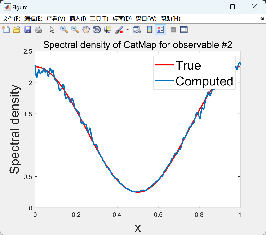
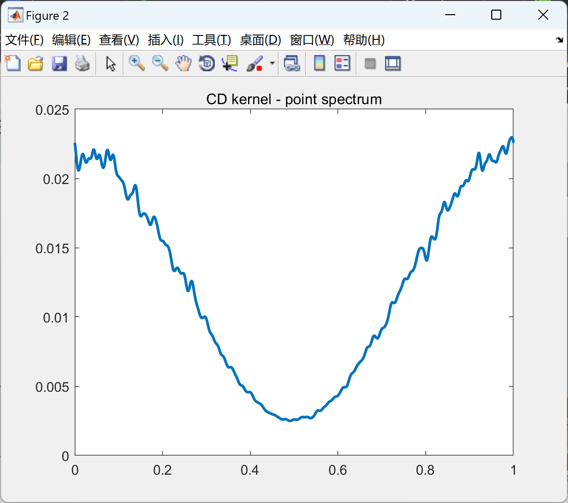
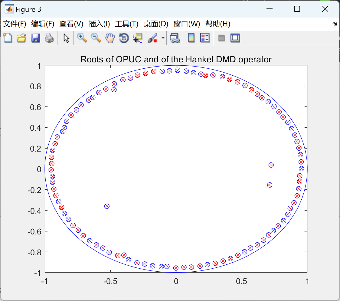
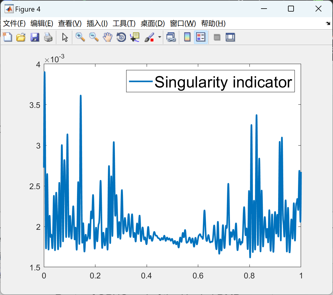
从测量数据开始,我们开发了一种方法来计算Koopman算子谱的细微结构,并提供了严格的收敛保证。该方法基于这样的观察:在保度测度的遍历设置中,与给定可观测量相关的谱测度的矩可以从该可观测量的单个轨迹中计算出来。有了有限数量的矩可用,我们使用经典的Christoffel-Darboux核来分离谱的原子部分和绝对连续部分,并且在矩的数量趋于无穷时支持收敛保证。此外,我们提出了一种技术来检测谱的奇异连续部分,以及两种近似谱测度的方法,在弱拓扑下保证收敛,无论奇异连续部分是否存在。所提出的方法易于实现,并且适用于大规模系统,因为计算复杂性主要由求解一个N×N的埃尔米特正定Toeplitz矩阵所主导,其中N是矩的数量,存在高效且数值稳定的算法;特别是,该方法的复杂性与底层状态空间的维度无关。我们还展示了如何从测量数据中计算出在单位圆上给定段的谱投影,从而获得明确考虑谱的点部分和连续部分的算子的有限逼近。最后,我们描述了所提出方法与所谓的Hankel动态模式分解之间的关系,提供了对Hankel DMD算子特征值行为的新见解。一些数值示例说明了该方法,包括对受盖板驱动的二维腔流的谱研究。
关键词:Koopman算子,谱分析,Christoffel-Darboux核,数据驱动方法,矩问题,Toeplitz矩阵。
光谱方法在大规模非线性动力系统的数据驱动分析中越来越受欢迎。其中,基于对Koopman算子的逼近的方法在各个领域取得了极大的成功。这个算子最初由Koopman [17] 几乎一个世纪前定义,是一个完全描述底层非线性动力系统的线性无限维算子。Koopman算子谱的逼近编码了有关底层系统动态的信息。例如,在[27]中分析了全局稳定性,而[28]处理了所谓的等稳线和等时线;在[7]中分析了遍历分区和混合性质,[18, 6]利用Koopman算子逼近进行控制,而[29]用于模型简化。最近的应用包括流体动力学[36, 2]、电力网络[32]、神经动力学[5]、能源效率[12]、分子物理学[48]和数据融合[47]。
自早期工作[29]以来,已经提出了许多用于逼近Koopman算子谱的算法,包括傅里叶平均值[29]和动态模式分解(DMD)的变体,例如[34, 47]。平均方法的好处在于它们有牢固的理论支持,具有强大的收敛结果;这种方法的局限性在于需要事先了解算子的特征值,并且这些方法不提供有关算子连续谱部分的任何信息。另一方面,类似DMD的方法不需要事先了解特征值,但它们的谱收敛性质不那么有利[19],并且与平均方法类似,它们不系统地处理谱的连续部分。另一种方法在[13]中进行,其中通过一个正则化的对流扩散算子计算Koopman特征函数。
本文提出了一种基于新的谐波分析、数据驱动方法来逼近Koopman算子谱的方法,能够计算谱的点部分和连续部分(并提供收敛保证),从而推广了[29]的方法。我们从这样一个观察开始:在保度遍历设置中,与给定可观测量相关的谱测度的矩可以从该可观测量的单个轨迹中计算出来。因此,在这种情况下,逼近Koopman算子的谱的问题归结为从其矩重建测度的问题。由于算子是酉的,测度支持在复平面中的单位圆上,这是一个非常理解的设置,最早的结果可以追溯到经典傅里叶分析。在我们的工作中,我们利用了这一领域的现代结果在Koopman算子设置中。我们主要依赖于Christoffel-Darboux核,它允许我们逼近谱的原子部分(即特征值)以及绝对连续部分。
详细文章见第4部分。
📚2 运行结果
部分代码:
figure(),clf
subplot(2,2,1)
plot(theta,r1,'k','LineWidth',2),hold on
plot(linspace(0,2*pi,L),phi1,'--','LineWidth',2)
xlim([0,2*pi]), xlabel('$\theta$'), legend('analytical','Welch')
title('cat map, $\rho(g_1)$')
subplot(2,2,2)
plot(theta,r2,'k','LineWidth',2),hold on
plot(linspace(0,2*pi,L),phi2,'--','LineWidth',2)
xlim([0,2*pi]), xlabel('$\theta$'), legend('analytical','Bartlett')
title('cat map, $\rho(g_2)$')
subplot(2,2,3)
semilogy(linspace(0,2*pi*fs,L),phi3/fs,'LineWidth',2) % we have to scale according to sampling frequency
xlim([0 fs*pi])
title('Lorenz, $\rho(x_1)$'), xlabel('$\omega$')
legend('Welch')
subplot(2,2,4)
semilogy(linspace(0,ws,L),phi4*2*pi/ws,'LineWidth',2) % we have to scale according to sampling frequency
xlim([0 ws/2])
title('cavity random observable, $\rho(\psi_1)$'),xlabel('$\omega$')
legend('Welch')
end
function [Y]=LorenzData(dt,n)
%% creates samples of data from Lorenz chaotic attractor
% dt : sampling interval
% n : number of samples
% Lorenz chaotic model 1963
sigma=10;
rho = 28;
beta = 8/3;
Lorenz = @(x) [sigma*(x(2)-x(1)); ...
x(1)*(rho-x(3))-x(2);...
x(1)*x(2)-beta*x(3)];
tspan = 0:dt:(n*dt + 20); %% allow 20 seconds of transients
x0 = [0.1;0;0.1];
[tspan,Y]= ode45(@(t,y)Lorenz(y),tspan,x0);
Y = Y(tspan>20,:);
end
function [Y]=CatMapData(n)
%% creates samples of data from Arnold's cat map
% n : number of samples
X = zeros(2,n);
X(:,1)=[.2;.37];
for i=1:n-1
X(:,i+1)=mod([2 1; 1 1]*X(:,i),1);
end
🎉3 参考文献
文章中一些内容引自网络,会注明出处或引用为参考文献,难免有未尽之处,如有不妥,请随时联系删除。


 3792
3792

 被折叠的 条评论
为什么被折叠?
被折叠的 条评论
为什么被折叠?
 到【灌水乐园】发言


