（2-2）TensorFlow数据集制作实战：将模拟数据制作成内存对象数据集

2.2  将模拟数据制作成内存对象数据集实战

在人工智能迅速发展的今天， 已经出现了各种各样的深度学习框架， 我们知道，深度学习要基于大量的样本数据来训练模型，那么数据集的制作或选取就显得尤为重要。在本节的内容中，将详细讲解将模拟数据制作成内存对象数据集的知识。

2.2.1  可视化内存对象数据集

在下面的实例文件data01.py中，自定义创建了生成器函数generate_data()，功能是创建在-1到1之间连续的100个浮点数，然后在Matplotlib中可视化展示用这些浮点数构成的数据集。实例文件data01.py的具体实现代码如下所示。

import tensorflow as tf
import numpy as np
import matplotlib.pyplot as plt

plt.rcParams['font.sans-serif'] = ['SimHei']  # 显示中文标签
plt.rcParams['axes.unicode_minus'] = False  # 这两行需要手动设

print(tf.__version__)
print(np.__version__)


def generate_data(batch_size=100):
    """y = 2x 函数数据生成器"""
    x_batch = np.linspace(-1, 1, batch_size)  # 为-1到1之间连续的100个浮点数
    x_batch = tf.cast(x_batch, tf.float32)
    #     print("*x_batch.shape", *x_batch.shape)
    y_batch = 2 * x_batch + np.random.randn(x_batch.shape[0]) * 0.3  # y=2x，但是加入了噪声
    y_batch = tf.cast(y_batch, tf.float32)

    yield x_batch, y_batch  # 以生成器的方式返回

# 1.循环获取数据
train_epochs = 10
for epoch in range(train_epochs):
    for x_batch, y_batch in generate_data():
        print(epoch, "| x.shape:", x_batch.shape, "| x[:3]:", x_batch[:3].numpy())
        print(epoch, "| y.shape:", y_batch.shape, "| y[:3]:", y_batch[:3].numpy())

# 2.显示一组数据
train_data = list(generate_data())[0]
plt.plot(train_data[0], train_data[1], 'ro', label='Original data')
plt.legend()
plt.show()

执行后会输出下面的结果，并在Matplotlib中绘制可视化结果，如图2-1所示。

2.6.0
1.19.5
0 | x.shape: (100,) | x[:3]: [-1.         -0.97979796 -0.959596  ]
0 | y.shape: (100,) | y[:3]: [-1.9194145 -2.426661  -1.8962196]
1 | x.shape: (100,) | x[:3]: [-1.         -0.97979796 -0.959596  ]
1 | y.shape: (100,) | y[:3]: [-1.6366603 -2.1575317 -1.2637805]
2 | x.shape: (100,) | x[:3]: [-1.         -0.97979796 -0.959596  ]
2 | y.shape: (100,) | y[:3]: [-2.1715505 -1.7276137 -2.1352115]
3 | x.shape: (100,) | x[:3]: [-1.         -0.97979796 -0.959596  ]
3 | y.shape: (100,) | y[:3]: [-2.2009645 -1.969894  -1.9827154]
4 | x.shape: (100,) | x[:3]: [-1.         -0.97979796 -0.959596  ]
4 | y.shape: (100,) | y[:3]: [-1.8537583 -1.1212573 -1.7960321]
5 | x.shape: (100,) | x[:3]: [-1.         -0.97979796 -0.959596  ]
5 | y.shape: (100,) | y[:3]: [-1.5608777 -1.7441161 -1.8731359]
6 | x.shape: (100,) | x[:3]: [-1.         -0.97979796 -0.959596  ]
6 | y.shape: (100,) | y[:3]: [-1.6598525 -2.7624342 -2.126709 ]
7 | x.shape: (100,) | x[:3]: [-1.         -0.97979796 -0.959596  ]
7 | y.shape: (100,) | y[:3]: [-1.7708246 -1.8593228 -1.875349 ]
8 | x.shape: (100,) | x[:3]: [-1.         -0.97979796 -0.959596  ]
8 | y.shape: (100,) | y[:3]: [-2.0270834 -1.8438468 -1.7587183]
9 | x.shape: (100,) | x[:3]: [-1.         -0.97979796 -0.959596  ]
9 | y.shape: (100,) | y[:3]: [-1.9673357 -1.6247914 -1.8439946]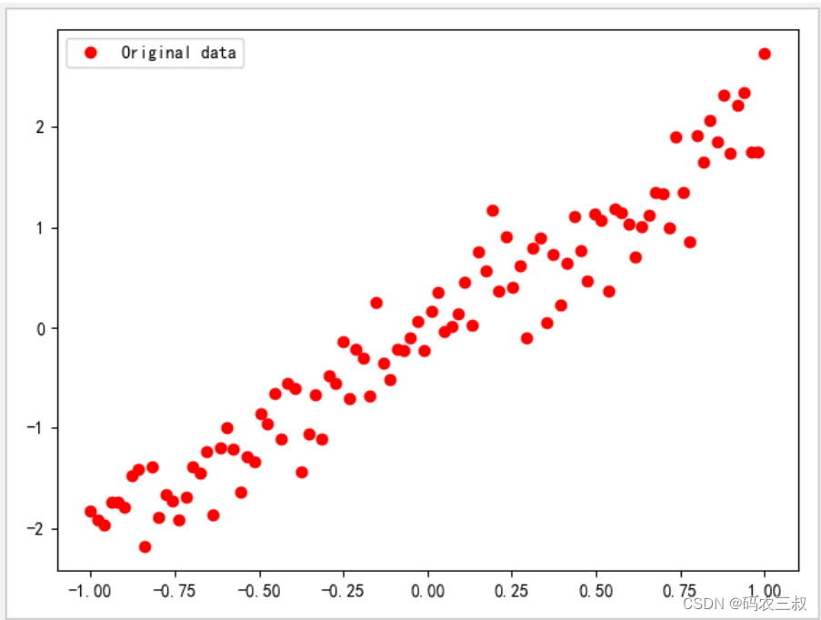

图2-1  可视化结果

通过上述输出结果可以看到，每次生成的x的数据都是一样的，这是由x的生成方式决定的， 如果你觉得这种数据不是你想要的，那么接下来可以生成乱序数据以消除这种影响，我们只需要对上述代码稍加修改即可。

2.2.2  改进的方案

在下面的实例文件data02.py中，通过添加迭代器的方式生成乱序数据，这样可以消除每次生成的x的数据都是一样的这种影响。实例文件data02.py的具体实现代码如下所示。

plt.rcParams['font.sans-serif'] = ['SimHei']  # 显示中文标签
plt.rcParams['axes.unicode_minus'] = False  # 这两行需要手动设

print(tf.__version__)
print(np.__version__)

def generate_data(epochs, batch_size=100):
    """y = 2x 函数数据生成器 增加迭代器"""
    for i in range(epochs):
        x_batch = np.linspace(-1, 1, batch_size)    # 为-1到1之间连续的100个浮点数
    #     print("*x_batch.shape", *x_batch.shape)
        y_batch = 2 * x_batch + np.random.randn(x_batch.shape[0]) * 0.3     # y=2x，但是加入了噪声

        yield shuffle(x_batch, y_batch), i        # 以生成器的方式返回

# 1.循环获取数据
train_epochs = 10

for (x_batch, y_batch), epoch_index in generate_data(train_epochs):
    x_batch = tf.cast(x_batch, tf.float32)
    y_batch = tf.cast(y_batch, tf.float32)
    print(epoch_index, "| x.shape:", x_batch.shape, "| x[:3]:", x_batch[:3].numpy())
    print(epoch_index, "| y.shape:", y_batch.shape, "| y[:3]:", y_batch[:3].numpy())

# 2.显示一组数据
train_data = list(generate_data(1))[0]
plt.plot(train_data[0][0], train_data[0][1], 'ro', label='Original data')
plt.legend()
plt.show()

此时执行后会输出下面的结果，会发现每次生成的x的数据都是不一样的。

2.6.0
1.19.5
0 | x.shape: (100,) | x[:3]: [-0.15151516  0.7171717   0.53535354]
0 | y.shape: (100,) | y[:3]: [0.05597204 1.304756   0.83463794]
1 | x.shape: (100,) | x[:3]: [-0.11111111 -0.5151515   0.83838385]
1 | y.shape: (100,) | y[:3]: [ 0.4798906 -1.1424009  1.1031219]
2 | x.shape: (100,) | x[:3]: [-0.8989899 -0.959596   0.8989899]
2 | y.shape: (100,) | y[:3]: [-2.444981  -1.5715022  1.3514851]
3 | x.shape: (100,) | x[:3]: [ 0.4949495   0.8181818  -0.03030303]
3 | y.shape: (100,) | y[:3]: [ 1.3379701   1.1126918  -0.11468022]
4 | x.shape: (100,) | x[:3]: [ 0.47474748 -0.21212122  0.5959596 ]
4 | y.shape: (100,) | y[:3]: [ 1.1210855  -0.90032357  1.3082465 ]
5 | x.shape: (100,) | x[:3]: [0.35353535 0.13131313 0.43434343]
5 | y.shape: (100,) | y[:3]: [ 0.7534245  -0.0981291   0.90445507]
6 | x.shape: (100,) | x[:3]: [-0.6969697  -0.21212122  0.8787879 ]
6 | y.shape: (100,) | y[:3]: [-1.4252775  -0.28825748  1.73506   ]
7 | x.shape: (100,) | x[:3]: [-0.67676765  0.21212122 -0.75757575]
7 | y.shape: (100,) | y[:3]: [-1.5350174  0.316071  -1.4615428]
8 | x.shape: (100,) | x[:3]: [ 0.15151516 -0.35353535  0.7979798 ]
8 | y.shape: (100,) | y[:3]: [ 0.6063673  -0.34562942  1.8686969 ]
9 | x.shape: (100,) | x[:3]: [-0.47474748  0.05050505 -0.7777778 ]
9 | y.shape: (100,) | y[:3]: [-1.398643    0.50217235 -1.5945572 ]

并且也会在Matplotlib中绘制可视化结果，如图2-2所示。

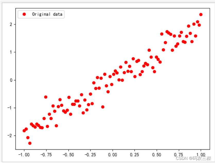
图2-2  可视化数据