


在之前的文章中,我们多次提及了OpenAI在大模型领域的领先优势,今天我们从数据分析的角度,来验证我们的结论。
排名可参考之前的文章:deepseek异军突起——2025年最新大模型排名-CSDN博客
或直接参考SuperCLUE数据来源。这里我们以总分榜来分析,并且假设,这些成绩是客观,合理的。
数据放在文章最后面,作图的代码也一并放在最后。
数据分析
我们先来做一个直方图,其中横轴是分数,纵轴是分数的频数。并且以左偏正态分布来拟合数据。
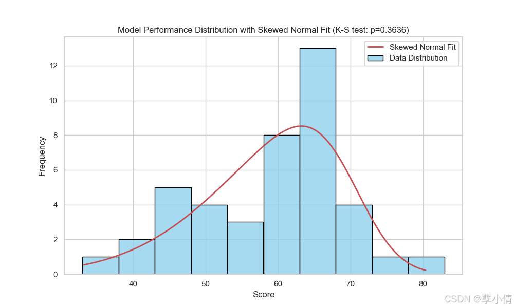
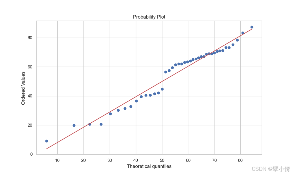
从拟合结果来看,还是比较符合左偏正态分布的,我们做Q-Q图看下:
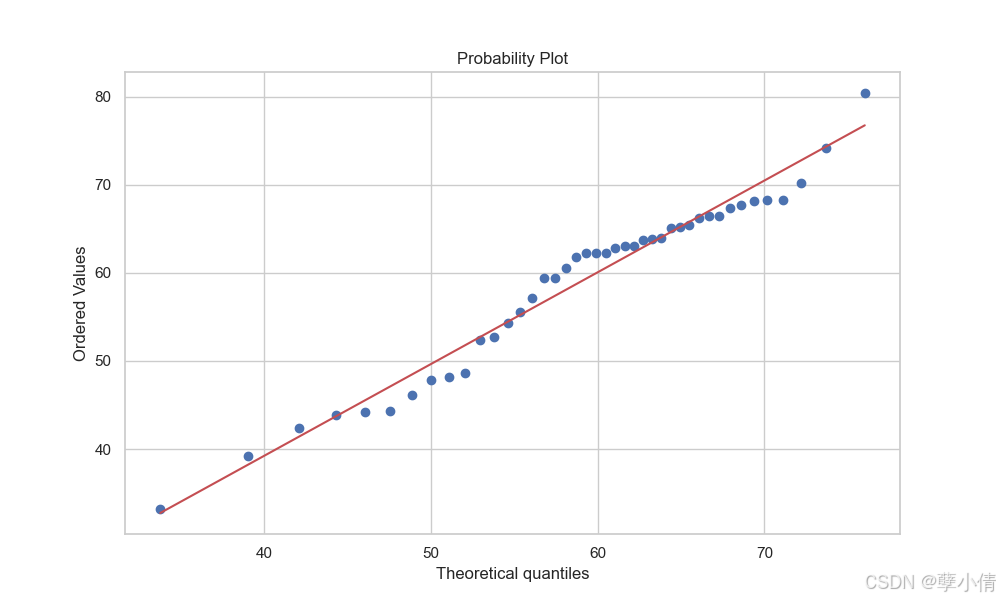
大致均匀分布于数据两侧,说明使用左偏正态分布拟合有一定合理性。接下来我们继续分析图表。
我们把分数70分作为一个分水岭,并在图中标出:
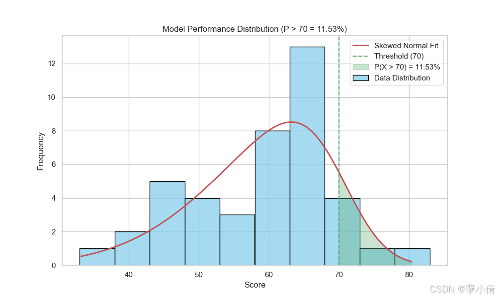
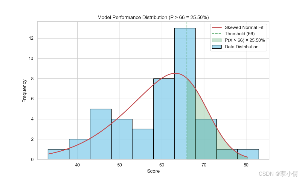
可以计算出,超过70分占比约11%,而这个顶尖的11%,他们同属于一个机构——OpenAI。豆包得分66.5分,如果我们以66分作为分界线,可以看到豆包大约在25%的位置,大概就是top4的水平,也相当不错了。只不过60分到70分之间竞争太激烈了,虽然豆包也占据了前几名的好成绩,但是领先优势不大。
我们再来选取理科成绩,其实理科成绩更好说明一点,因为理科成绩最高分87.3,最低分31.2,范围分布更宽,可能会更明显。
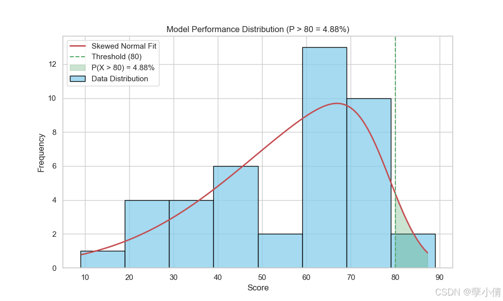
这次我们设置bin宽度为10,且同样以左偏正态分布拟合,选取80分为临界点计算高于80分的概率,数据结果图所示。这次依然很极端,超过80分只有o1及o1-preivew。众数分布在60分到80分之间,换句话说,如果哪家的分数低于六十分,在排名上就会掉到很后,尽管可能跟60分的模型差距并没有那么大。
代码源码
import numpy as np
import pandas as pd
import matplotlib.pyplot as plt
import seaborn as sns
from scipy.stats import skewnorm, kstest
import scipy.stats as stats
import matplotlib as mpl
import platform

# 设置中文字体
plt.rcParams['font.sans-serif'] = ['SimSun']  # 宋体
plt.rcParams['axes.unicode_minus'] = False
plt.rcParams['font.family'] = 'sans-serif'

def read_data(filename):
    names = []
    values = []
    with open(filename, 'r', encoding='utf-8') as f:
        for line in f:
            parts = line.strip().split()
            if len(parts) >= 2:
                name = parts[0]
                try:
                    # 提取数字部分
                    value_str = ''.join(c for c in parts[-1] if c.isdigit() or c == '.')
                    value = float(value_str)
                    names.append(name)
                    values.append(value)
                except ValueError:
                    print(f"Warning: Skipping invalid data line: {line.strip()}")
    return np.array(names), np.array(values)

def perform_ks_test(data, distribution, *params):
    """
    Perform Kolmogorov-Smirnov test for goodness of fit

    Parameters:
    -----------
    data : array-like
        Observed data
    distribution : scipy.stats distribution object
        The theoretical distribution to test against
    *params : tuple
        Parameters of the theoretical distribution

    Returns:
    --------
    dict
        Dictionary containing test statistic, p-value and test result
    """
    # Perform K-S test
    statistic, p_value = kstest(data, distribution.name, args=params)

    # Interpret results
    alpha = 0.05  # conventional significance level
    is_good_fit = p_value > alpha

    result = {
        'statistic': statistic,
        'p_value': p_value,
        'is_good_fit': is_good_fit,
        'alpha': alpha
    }

    return result

def calculate_exceedance_probability(distribution, params, threshold):
    """
    Calculate the probability of exceeding a threshold value

    Parameters:
    -----------
    distribution : scipy.stats distribution object
        The fitted distribution
    params : tuple
        Parameters of the distribution (a, loc, scale)
    threshold : float
        The threshold value

    Returns:
    --------
    float
        Probability of exceeding the threshold
    """
    # Calculate survival function (1 - CDF)
    prob = 1 - distribution.cdf(threshold, *params)
    return prob

def plot_histogram_with_normal_fit(values, title="Model Performance Distribution", num_bins=10, bin_width=None, threshold=80):
    if bin_width is not None:
        # 如果指定了bin宽度,则使用它来创建bins
        min_val = np.floor(min(values))
        max_val = np.ceil(max(values))
        bins = np.arange(min_val, max_val + bin_width, bin_width)
        num_bins = len(bins) - 1  # 计算实际的bin数量
    else:
        # 如果没有指定bin宽度,则使用指定的bin数量
        bins = num_bins

    # 使用最大似然估计拟合偏正态分布参数
    # skewnorm.fit返回三个参数:a (偏度参数),loc (位置参数),scale (尺度参数)
    a, loc, scale = skewnorm.fit(values)
    print(f"Fitted Parameters:\n  Skewness (a) = {a:.2f}\n  Location (loc) = {loc:.2f}\n  Scale (scale) = {scale:.2f}")

    # Calculate probability of exceeding threshold
    exceed_prob = calculate_exceedance_probability(skewnorm, (a, loc, scale), threshold)
    print(f"\nProbability Analysis:")
    print(f"  Probability of scoring above {threshold}: {exceed_prob:.2%}")

    # Calculate actual percentage in data
    actual_exceed = np.mean(values > threshold)
    print(f"  Actual percentage above {threshold} in data: {actual_exceed:.2%}")

    # Perform K-S test
    ks_result = perform_ks_test(values, skewnorm, a, loc, scale)
    print("\nKolmogorov-Smirnov Test Results:")
    print(f"  Statistic (D) = {ks_result['statistic']:.4f}")
    print(f"  p-value = {ks_result['p_value']:.4f}")
    print(f"  Significance level (α) = {ks_result['alpha']}")
    print(f"  Conclusion: The data {'is' if ks_result['is_good_fit'] else 'is not'} well-fitted by the skewed normal distribution")

    # 设置 Seaborn 风格
    sns.set(style="whitegrid")
    plt.figure(figsize=(10, 6))

    # 使用 seaborn 的 histplot 绘制频数直方图
    sns.histplot(
        x=values,
        bins=bins,
        kde=False,
        stat='count',
        color='skyblue',
        edgecolor='black',
        label='Data Distribution'
    )

    # 生成用于绘制 PDF 的 x 坐标
    x_pdf = np.linspace(values.min(), values.max(), 100)
    pdf = skewnorm.pdf(x_pdf, a, loc, scale)

    # 计算bin宽度和缩放系数
    bin_width_actual = (values.max() - values.min()) / num_bins
    print(f"\nBin width: {bin_width_actual}")

    # PDF × (总样本数 × bin宽度) = "频数"级别下的 PDF
    pdf_scaled = pdf * len(values) * bin_width_actual

    print(f"pdf_scaled shape: {pdf_scaled.shape}, x_pdf shape: {x_pdf.shape}")

    # 绘制缩放后的 PDF
    plt.plot(x_pdf, pdf_scaled, 'r-', lw=2, label='Skewed Normal Fit')

    # Add vertical line for threshold
    plt.axvline(x=threshold, color='g', linestyle='--', label=f'Threshold ({threshold})')

    # Add shaded area for scores above threshold
    x_shade = np.linspace(threshold, values.max(), 50)
    pdf_shade = skewnorm.pdf(x_shade, a, loc, scale) * len(values) * bin_width_actual
    plt.fill_between(x_shade, pdf_shade, alpha=0.3, color='g',
                    label=f'P(X > {threshold}) = {exceed_prob:.2%}')

    # Add K-S test result and probability to the plot title
    title_text = f"Model Performance Distribution (P > {threshold} = {exceed_prob:.2%})"
    plt.title(title_text)
    plt.xlabel('Score')
    plt.ylabel('Frequency')
    plt.legend()

    # 保存图片
    plt.savefig('histogram.png')
    plt.close()

    plt.figure(figsize=(10, 6))
    plt.title('Q-Q 图:成绩数据与伽马分布拟合')
    plt.xlabel('Expected Quantiles')
    plt.ylabel('Sample Quantiles')
    stats.probplot(values, dist="skewnorm", sparams=(a, loc, scale), plot=plt)
    plt.savefig('qq.png')
    plt.close()

def main():
    try:
        # 读取数据
        names, values = read_data('data.txt')

        num_bins = None
        bin_width = 5

        # 绘制直方图并拟合左偏正态分布
        plot_histogram_with_normal_fit(values, num_bins=num_bins, bin_width=bin_width)
        print("Histogram has been generated and saved as 'histogram.png'")
        if bin_width:
            print(f"Used bin width: {bin_width}")
        else:
            print(f"Used number of bins: {num_bins}")

        # 输出基本统计信息
        print(f"\nBasic Statistics:")
        print(f"Mean: {np.mean(values):.2f}")
        print(f"Standard Deviation: {np.std(values):.2f}")
        print(f"Median: {np.median(values):.0f}")

    except FileNotFoundError:
        print("Error: data.txt file not found")
    except Exception as e:
        print(f"An error occurred: {str(e)}")

if __name__ == "__main__":
    main()
SuperCLUE总排行榜(2024年12月)
| 排名 | 模型名称 | 机构 | 总分 | Hard | 理科 | 文科 | 使用方式 | 发布日期 |
|---|---|---|---|---|---|---|---|---|
| - | o1 | OpenAI | 80.4 | 76.7 | 87.3 | 77.1 | 网页 | 2025年1月8日 |
| - | o1-preview | OpenAI | 74.2 | 63.6 | 80.6 | 78.5 | API | 2025年1月8日 |
| - | ChatGPT-4o-latest | OpenAI | 70.2 | 57.8 | 72.1 | 80.7 | API | 2025年1月8日 |
| 🏅️ | DeepSeek-V3 | 深度求索 | 68.3 | 54.8 | 72 | 78.2 | API | 2025年1月8日 |
| 🏅️ | SenseChat 5.5-latest | 商汤 | 68.3 | 51.5 | 71.6 | 81.8 | API | 2025年1月8日 |
| - | Gemini-2.0-Flash-Exp | | 68.2 | 55.5 | 72.6 | 76.6 | API | 2025年1月8日 |
| - | Claude 3.5 Sonnet(20241022) | Anthropic | 67.7 | 54.6 | 71.4 | 77.2 | API | 2025年1月8日 |
| 🏅️ | 360zhinao2-o1 | 360 | 67.4 | 51.4 | 72.1 | 78.7 | API | 2025年1月8日 |
| 🥈 | Doubao-pro-32k-241215 | 字节跳动 | 66.5 | 50.6 | 72.3 | 76.6 | API | 2025年1月8日 |
| 🥈 | NebulaCoder-V5 | 中兴通讯 | 66.4 | 48.6 | 69.5 | 80.9 | API | 2025年1月8日 |
| 🥈 | Qwen-max-latest | 阿里巴巴 | 66.2 | 51.3 | 67.4 | 80 | API | 2025年1月8日 |
| - | Qwen2.5-72B-Instruct | 阿里巴巴 | 65.4 | 49.7 | 66.2 | 80.3 | API | 2025年1月8日 |
| 🥉 | Step-2-16k | 阶跃星辰 | 65.2 | 50 | 65.1 | 80.3 | API | 2025年1月8日 |
| 🥉 | GLM-4-Plus | 智谱AI | 65.1 | 48.5 | 68.1 | 78.8 | API | 2025年1月8日 |
| - | Grok-2-1212 | X.AI | 63.9 | 49.2 | 66.8 | 75.5 | API | 2025年1月8日 |
| - | DeepSeek-R1-Lite-Preview | 深度求索 | 63.8 | 44.9 | 69.7 | 76.8 | 网页 | 2025年1月8日 |
| - | Qwen2.5-32B-Instruct | 阿里巴巴 | 63.7 | 44.9 | 66.9 | 79.1 | API | 2025年1月8日 |
| 4 | Sky-Chat-3.0 | 昆仑万维 | 63 | 44.5 | 65.4 | 79.1 | API | 2025年1月8日 |
| - | DeepSeek-V2.5 | 深度求索 | 63 | 45.3 | 67.6 | 76.1 | API | 2025年1月8日 |
| 4 | MiniMax-abab7-preview | MiniMax | 62.8 | 42.8 | 64.9 | 80.7 | API | 2025年1月8日 |
| 4 | Hunyuan-Turbo | 腾讯 | 62.3 | 38.6 | 67.7 | 80.6 | API | 2025年1月8日 |
| 4 | TeleChat2-Large | TeleAI | 62.3 | 43.3 | 64.1 | 79.5 | API | 2025年1月8日 |
| 4 | ERNIE-4.0-Turbo-8K-Latest | 百度 | 62.2 | 45.6 | 61.4 | 79.5 | API | 2025年1月8日 |
| 5 | Baichuan4 | 百川智能 | 61.8 | 45 | 62 | 78.2 | API | 2025年1月8日 |
| - | GPT-4o-mini | OpenAI | 60.6 | 42.8 | 63.3 | 75.8 | API | 2025年1月8日 |
| 6 | kimi | Kimi | 59.4 | 43.5 | 58.1 | 76.6 | 网页 | 2025年1月8日 |
| - | Llama-3.3-70B-Instruct | Meta | 59.4 | 38.8 | 66.4 | 72.9 | API | 2025年1月8日 |
| 7 | TeleChat2-35B | TeleAI | 57.1 | 37.6 | 55.6 | 78.2 | 模型 | 2025年1月8日 |
| 8 | Qwen2.5-7B-Instruct | 阿里巴巴 | 55.5 | 35.7 | 54.4 | 76.4 | API | 2025年1月8日 |
| 9 | QwQ-32B-Preview | 阿里巴巴 | 54.3 | 26.6 | 59.8 | 76.5 | API | 2025年1月8日 |
| 10 | 讯飞星火V4.0 | 科大讯飞 | 52.7 | 20.3 | 62.3 | 75.4 | API | 2025年1月8日 |
| 10 | GLM-4-9B-Chat | 智谱AI | 52.4 | 31.6 | 50.6 | 75.1 | 模型 | 2025年1月8日 |
| - | Gemma-2-9b-it | | 48.6 | 22.7 | 49.5 | 73.7 | 模型 | 2025年1月8日 |
| 11 | Yi-1.5-34B-Chat-16K | 零一万物 | 48.2 | 20.6 | 48.2 | 75.9 | 模型 | 2025年1月8日 |
| 11 | 360Zhinao2-7B-Chat-4K | 360 | 47.8 | 17.5 | 50.7 | 75.2 | 模型 | 2025年1月8日 |
| 12 | Qwen2.5-3B-Instruct | 阿里巴巴 | 46.1 | 18.6 | 44.2 | 75.5 | API | 2025年1月8日 |
| 13 | Yi-1.5-9B-Chat-16K | 零一万物 | 44.3 | 20.3 | 41.3 | 71.3 | 模型 | 2025年1月8日 |
| 13 | MiniCPM3-4B | 面壁智能 | 44.2 | 13.7 | 45.9 | 73 | 模型 | 2025年1月8日 |
| - | Llama-3.1-8B-Instruct | Meta | 43.9 | 20.9 | 42.8 | 68.1 | API | 2025年1月8日 |
| - | Phi-3.5-Mini-Instruct | 微软 | 42.4 | 14 | 42.4 | 70.7 | 模型 | 2025年1月8日 |
| - | Gemma-2-2b-it | | 39.2 | 11.8 | 36.4 | 69.4 | 模型 | 2025年1月8日 |
| - | Mistral-7B-Instruct-v0.3 | Mistral AI | 33.2 | 11.4 | 31.2 | 56.9 | 模型 | 2025年1月8日 |


 3757
3757

 被折叠的 条评论
为什么被折叠?
被折叠的 条评论
为什么被折叠?
 到【灌水乐园】发言


