物理学视角讲解diffusion生成模型——隐扩散模型

最新推荐文章于 2024-07-13 17:48:20 发布

远洋之帆

最新推荐文章于 2024-07-13 17:48:20 发布

阅读量1k

点赞数 14

文章标签：人工智能机器学习自然语言处理搜索引擎

本文链接：https://blog.csdn.net/liangwqi/article/details/138030808

版权

https://zhuanlan.zhihu.com/p/692996885
https://zhuanlan.zhihu.com/p/693255617
前面两篇文章介绍了扩散过程，同时实现了1维、2维混合高斯扩散、逆扩散，通过模型预测得分函数来实现逆扩散推理。这个章节介绍工业界使用的文本生成图扩撒模型：stable diffusion。

学习生成新内容的方法（正向/逆向扩散）
将文本与图像关联的方式（如CLIP的文图表示模型）
压缩图像的方式（自动编码器）
与学习评分函数相关的损失
用于处理图像的U-Net架构
加入控制条件方式（U-net架构 + 自我/交叉注意力）

后面章节会将上述每个部分的一些内容代码实现，到最后将拥有一个运行中的类Stable-Diffusion模型。

基础知识

让我们从正向扩散开始。在最简单的情况下，相关的扩散方程是：
$KaTeX parse error: {equation} can be used only in display mode.$
其中 $\sigma(t) > 0$ 是“噪声强度”， $\Delta t$ 是步长， $\sim \mathcal{N}(0, 1)$ 是一个标准正态随机变量。本质上，我们不断地向样本中添加正态分布的噪声。通常，噪声强度 $\sigma(t)$ 会随时间变化（即随着 t$的增大而增大）。
我们可以通过一个类似的更新规则来逆转这个扩散过程：
$KaTeX parse error: {equation} can be used only in display mode.$
被称为得分函数。如果我们知道这个函数，我们可以逆转正向扩散，并将噪声还原为我们开始时的状态。
如果我们的初始样本始终只有一个点 $x_0 = 0$ ，并且噪声强度是恒定的，那么得分函数就等于
$KaTeX parse error: {equation} can be used only in display mode.$
然后通常情况，我们并不事先知道得分函数；相反，我们需要学习它。一种学习它的方法是通过去噪目标训练一个神经网络来`去噪’样本。
$KaTeX parse error: {equation} can be used only in display mode.$
其中 $p_0(x_0)$ 是我们的目标分布（例如猫和狗的图片）， $x_{noised}$ 是目标分布样本 $x_0$ 经过一步正向扩散后的状态，即 $x_{noised} - x_0$ 只是一个正态分布的随机变量。
这里有另一种写法，更接近实际实现：
$KaTeX parse error: {equation} can be used only in display mode.$

像素空间扩散模型

无条件约束扩散模型

通过U型网络处理图像

前面回顾了扩散模型的基础知识，关键在于学习得分函数可以让我们将纯噪声转变为想要的东西。我们将用神经网络来近似得分函数。但当我们处理图像时，我们需要我们的神经网络与它们“友好相处”，并反映出感应…空间尺度。
由于得分函数是时间的函数，我们还需要找到一种方法确保我们的神经网络能够正确响应时间的变化。为此，我们可以使用时间嵌入。
下面的代码通过时间嵌入让神经网络处理时间。其思想是，不仅仅告诉网络一个数字（当前时间），而是用许多正弦特征来表达当前时间。以多种不同的方式告诉网络当前的时间，它将更容易地响应时间的变化。
这将使神经网络能够成功学习一个与时间相关的得分函数s(x, t)。

#@title Get some modules to let time interact

class GaussianFourierProjection(nn.Module):
    """Gaussian random features for encoding time steps."""  
    def __init__(self, embed_dim, scale=30.):
        super().__init__()
        # Randomly sample weights (frequencies) during initialization. 
        # These weights (frequencies) are fixed during optimization and are not trainable.
        self.W = nn.Parameter(torch.randn(embed_dim // 2) * scale, requires_grad=False)
    def forward(self, x):
        # Cosine(2 pi freq x), Sine(2 pi freq x)
        x_proj = x[:, None] * self.W[None, :] * 2 * np.pi
        return torch.cat([torch.sin(x_proj), torch.cos(x_proj)], dim=-1)


class Dense(nn.Module):
    """A fully connected layer that reshapes outputs to feature maps.
  Allow time repr to input additively from the side of a convolution layer.
  """
    def __init__(self, input_dim, output_dim):
        super().__init__()
        self.dense = nn.Linear(input_dim, output_dim)
    def forward(self, x):
        return self.dense(x)[..., None, None] 
# this broadcast the 2d tensor to 4d, add the same value across space.

定义U-Net架构

#@title Defining a time-dependent score-based model (double click to expand or collapse)

class UNet(nn.Module):
  """A time-dependent score-based model built upon U-Net architecture."""

  def __init__(self, marginal_prob_std, channels=[32, 64, 128, 256], embed_dim=256):
    """Initialize a time-dependent score-based network.

    Args:
      marginal_prob_std: A function that takes time t and gives the standard
        deviation of the perturbation kernel p_{0t}(x(t) | x(0)).
      channels: The number of channels for feature maps of each resolution.
      embed_dim: The dimensionality of Gaussian random feature embeddings.
    """
    super().__init__()
    # Gaussian random feature embedding layer for time
    self.time_embed = nn.Sequential(
          GaussianFourierProjection(embed_dim=embed_dim),
          nn.Linear(embed_dim, embed_dim)
          )
    # Encoding layers where the resolution decreases
    self.conv1 = nn.Conv2d(1, channels[0], 3, stride=1, bias=False)
    self.dense1 = Dense(embed_dim, channels[0])
    self.gnorm1 = nn.GroupNorm(4, num_channels=channels[0])

    self.conv2 = nn.Conv2d(channels[0], channels[1], 3, stride=2, bias=False)
    self.dense2 = Dense(embed_dim, channels[1])
    self.gnorm2 = nn.GroupNorm(32, num_channels=channels[1])
    
    self.conv3 = nn.Conv2d(channels[1], channels[2], 3, stride=2, bias=False)
    self.dense3 = Dense(embed_dim, channels[2])
    self.gnorm3 = nn.GroupNorm(32, num_channels=channels[2])
    
    self.conv4 = nn.Conv2d(channels[2], channels[3], 3, stride=2, bias=False)
    self.dense4 = Dense(embed_dim, channels[3])
    self.gnorm4 = nn.GroupNorm(32, num_channels=channels[3])   
     

    # Decoding layers where the resolution increases
    self.tconv4 = nn.ConvTranspose2d(channels[3], channels[2], 3, stride=2, bias=False)
    self.dense5 = Dense(embed_dim, channels[2])
    self.tgnorm4 = nn.GroupNorm(32, num_channels=channels[2])
    self.tconv3 = nn.ConvTranspose2d(channels[2] + channels[2], channels[1], 3, stride=2, bias=False, output_padding=1)    
    self.dense6 = Dense(embed_dim, channels[1])
    self.tgnorm3 = nn.GroupNorm(32, num_channels=channels[1])
    self.tconv2 = nn.ConvTranspose2d(channels[1] + channels[1], channels[0], 3, stride=2, bias=False, output_padding=1)    
    self.dense7 = Dense(embed_dim, channels[0])
    self.tgnorm2 = nn.GroupNorm(32, num_channels=channels[0])
    self.tconv1 = nn.ConvTranspose2d(channels[0] + channels[0], 1, 3, stride=1)
    
    # The swish activation function
    self.act = lambda x: x * torch.sigmoid(x)
    self.marginal_prob_std = marginal_prob_std
  
  def forward(self, x, t, y=None): 
    # Obtain the Gaussian random feature embedding for t   
    embed = self.act(self.time_embed(t))    
    # Encoding path
    h1 = self.conv1(x)  + self.dense1(embed)   
    ## Incorporate information from t
    ## Group normalization
    h1 = self.act(self.gnorm1(h1))
    h2 = self.conv2(h1) + self.dense2(embed)
    h2 = self.act(self.gnorm2(h2))
    
    #   apply activation function
    h3 = self.conv3(h2) + self.dense3(embed)
    h3 = self.act(self.gnorm3(h3))
   
    h4 = self.conv4(h3) + self.dense4(embed)
    h4 = self.act(self.gnorm4(h4))

    # Decoding path
    h = self.tconv4(h4)
    ## Skip connection from the encoding path
    h += self.dense5(embed)
    h = self.act(self.tgnorm4(h))
    h = self.tconv3(torch.cat([h, h3], dim=1))
    h += self.dense6(embed)
    h = self.act(self.tgnorm3(h))
    h = self.tconv2(torch.cat([h, h2], dim=1))
    h += self.dense7(embed)
    h = self.act(self.tgnorm2(h))
    h = self.tconv1(torch.cat([h, h1], dim=1))

    # Normalize output
    h = h / self.marginal_prob_std(t)[:, None, None, None]
    return h

训练U-Net学习得分函数

将上面定义的U-Net与学习评分函数的方法结合起来。需要定义一个损失函数，然后以常规方式训练一个神经网络。
$\sigma^t dw$
该过程将噪声加到x样本上，噪声规模呈指数增长。
鉴于这一前向过程，以及给定一个起始x(0)，我们有一个解析解用于任何时间x(t)的样本
$p(x(t)|x(0))=\mathcal N(x(0),\sigma(t)^2)$
我们称 $\sigma(t)$ 为边际标准差，即条件分布的标准差。在这个特定情况下，
$\sigma^2(t)=\int_0^t (\sigma^\tau ) ^2d\tau = \int_0^t \sigma^{2\tau} d\tau = \frac{\sigma^{2t}-1}{2\log \sigma }$

扩散常数和噪声强度

#@title Diffusion constant and noise strength
device = 'cuda' #@param ['cuda', 'cpu'] {'type':'string'}

def marginal_prob_std(t, sigma):
    """Compute the mean and standard deviation of $p_{0t}(x(t) | x(0))$.

  Args:    
    t: A vector of time steps.
    sigma: The $\sigma$ in our SDE.  
  
  Returns:
    The standard deviation.
  """    
    t = torch.tensor(t, device=device)
    return torch.sqrt((sigma**(2 * t) - 1.) / 2. / np.log(sigma))

def diffusion_coeff(t, sigma):
    """Compute the diffusion coefficient of our SDE.

  Args:
    t: A vector of time steps.
    sigma: The $\sigma$ in our SDE.
  
  Returns:
    The vector of diffusion coefficients.
  """
    return torch.tensor(sigma**t, device=device)

sigma =  25.0#@param {'type':'number'}
marginal_prob_std_fn = functools.partial(marginal_prob_std, sigma=sigma)
diffusion_coeff_fn = functools.partial(diffusion_coeff, sigma=sigma)

定义损失函数

损失函数主要在下面定义。用强度为std[:, None, None, None]的随机噪声进行采样，并确保其形状与𝐱相同。然后使用这个来扰动𝐱。

def loss_fn(model, x, marginal_prob_std, eps=1e-5):
  """The loss function for training score-based generative models.

  Args:
    model: A PyTorch model instance that represents a 
      time-dependent score-based model.
    x: A mini-batch of training data.    
    marginal_prob_std: A function that gives the standard deviation of 
      the perturbation kernel.
    eps: A tolerance value for numerical stability.
  """
  # Sample time uniformly in 0, 1
  random_t = torch.rand(x.shape[0], device=x.device) * (1. - eps) + eps 
  # Find the noise std at the time `t`
  std = marginal_prob_std(random_t)
  
  z = torch.randn_like(x)             # get normally distributed noise
  perturbed_x = x + z * std[:, None, None, None]
  
  score = model(perturbed_x, random_t) #用模型来预测得分函数值
  loss = torch.mean(torch.sum((score * std[:, None, None, None] + z)**2, dim=(1,2,3)))
  return loss

定义采样器

#@title Sampler code
num_steps = 500#@param {'type':'integer'}
def Euler_Maruyama_sampler(score_model, 
              marginal_prob_std,
              diffusion_coeff, 
              batch_size=64, 
              x_shape=(1, 28, 28),
              num_steps=num_steps, 
              device='cuda', 
              eps=1e-3, y=None):
  """Generate samples from score-based models with the Euler-Maruyama solver.

  Args:
    score_model: A PyTorch model that represents the time-dependent score-based model.
    marginal_prob_std: A function that gives the standard deviation of
      the perturbation kernel.
    diffusion_coeff: A function that gives the diffusion coefficient of the SDE.
    batch_size: The number of samplers to generate by calling this function once.
    num_steps: The number of sampling steps. 
      Equivalent to the number of discretized time steps.
    device: 'cuda' for running on GPUs, and 'cpu' for running on CPUs.
    eps: The smallest time step for numerical stability.
  
  Returns:
    Samples.    
  """
  t = torch.ones(batch_size, device=device)
  init_x = torch.randn(batch_size, *x_shape, device=device) \
    * marginal_prob_std(t)[:, None, None, None]
  time_steps = torch.linspace(1., eps, num_steps, device=device)
  step_size = time_steps[0] - time_steps[1]
  x = init_x
  with torch.no_grad():
    for time_step in tqdm(time_steps):      
      batch_time_step = torch.ones(batch_size, device=device) * time_step
      g = diffusion_coeff(batch_time_step)
      mean_x = x + (g**2)[:, None, None, None] * score_model(x, batch_time_step, y=y) * step_size
      x = mean_x + torch.sqrt(step_size) * g[:, None, None, None] * torch.randn_like(x)      
  # Do not include any noise in the last sampling step.
  return mean_x

整合训练链路

把上面的各模块整合起来，用来MNIST数据来做无监督训练。

#@title Training the alternate U-Net model (double click to expand or collapse)

score_model = torch.nn.DataParallel(UNet_res(marginal_prob_std=marginal_prob_std_fn))
score_model = score_model.to(device)

n_epochs =   75#@param {'type':'integer'}
## size of a mini-batch
batch_size =  1024 #@param {'type':'integer'}
## learning rate
lr=10e-4 #@param {'type':'number'}

dataset = MNIST('.', train=True, transform=transforms.ToTensor(), download=True)
data_loader = DataLoader(dataset, batch_size=batch_size, shuffle=True, num_workers=4)

optimizer = Adam(score_model.parameters(), lr=lr)
scheduler = LambdaLR(optimizer, lr_lambda=lambda epoch: max(0.2, 0.98 ** epoch))
tqdm_epoch = trange(n_epochs)
for epoch in tqdm_epoch:
  avg_loss = 0.
  num_items = 0
  for x, y in data_loader:
    x = x.to(device)    
    loss = loss_fn(score_model, x, marginal_prob_std_fn)
    optimizer.zero_grad()
    loss.backward()    
    optimizer.step()
    avg_loss += loss.item() * x.shape[0]
    num_items += x.shape[0]
  scheduler.step()
  lr_current = scheduler.get_last_lr()[0]
  print('{} Average Loss: {:5f} lr {:.1e}'.format(epoch, avg_loss / num_items, lr_current))
  # Print the averaged training loss so far.
  tqdm_epoch.set_description('Average Loss: {:5f}'.format(avg_loss / num_items))
  # Update the checkpoint after each epoch of training.
  torch.save(score_model.state_dict(), 'ckpt_res.pth')

训练结果可视化

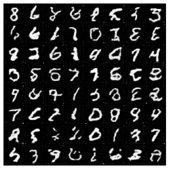
def save_samples_uncond(score_model, suffix=""):
  score_model.eval()
  ## Generate samples using the specified sampler.
  sample_batch_size = 64 #@param {'type':'integer'}
  num_steps = 250 #@param {'type':'integer'}
  sampler = Euler_Maruyama_sampler #@param ['Euler_Maruyama_sampler', 'pc_sampler', 'ode_sampler'] {'type': 'raw'}
  # score_model.eval()
  ## Generate samples using the specified sampler.
  samples = sampler(score_model, 
          marginal_prob_std_fn,
          diffusion_coeff_fn, 
          sample_batch_size, 
          num_steps=num_steps,
          device=device,
          )

      ## Sample visualization.
  samples = samples.clamp(0.0, 1.0)
  sample_grid = make_grid(samples, nrow=int(np.sqrt(sample_batch_size)))
  sample_np = sample_grid.permute(1, 2, 0).cpu().numpy()
  plt.imsave(f"uncondition_diffusion{suffix}.png", sample_np,)
  plt.figure(figsize=(6,6))
  plt.axis('off')
  plt.imshow(sample_np, vmin=0., vmax=1.)
  plt.show()

uncond_score_model = torch.nn.DataParallel(UNet_res(marginal_prob_std=marginal_prob_std_fn))
uncond_score_model.load_state_dict(torch.load("ckpt_res.pth"))
save_samples_uncond(uncond_score_model, suffix="_res")

带条件约束扩散模型

注意力机制实现条件生成扩散模型

除了生成数字0-9的图像外，我们还想进行条件生成：例如，我们想指定我们想生成哪个数字的图像。
注意力模型虽然对于条件生成来说不是绝对必要的，但已被证明对于使其良好工作非常有用。所以这部分我们会用注意模型来实现条件生成扩散模型。

文本控制条件

在这里，我们没有使用复杂的CLIP模型，而是定义了数字0-9的自己的向量表示。
我们使用了nn.Embedding层将0-9的索引转换成向量。

class WordEmbed(nn.Module):
  def __init__(self, vocab_size, embed_dim):
    super(WordEmbed, self).__init__()
    self.embed = nn.Embedding(vocab_size+1, embed_dim)
  
  def forward(self, ids):
    return self.embed(ids)

文本条件引入注意力模型

我们通常使用三个部分来实现注意力模型：

CrossAttention 编写一个模块来执行序列的自注意力/交叉注意力。
TransformerBlock 结合自注意力/交叉注意力和前馈神经网络。
SpatialTransformer 在U-net中使用注意力，将空间张量转换为序列张量，然后再转换回来。

实现CrossAttention类的一部分，并且还将在U-Net中添加注意力的位置。

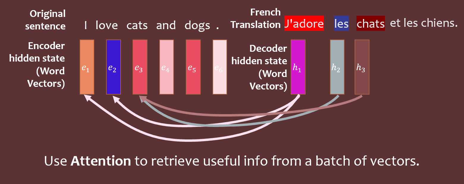
简要回顾一下注意力模型的数学原理。QKV（查询-键-值）注意力模型将查询、键和值表示为向量。这些工具帮助我们将翻译任务一侧的词语/图像与另一侧相关联。
这些向量与𝐞向量（代表编码器的隐藏状态）和𝐡向量（代表解码器的隐藏状态）线性相关：
$KaTeX parse error: {equation} can be used only in display mode.$
为了确定要“关注”什么，计算每个键𝐤和查询𝐪的内积（即相似性）。为了得到不太大也不太小的典型值，可以通过查询向量𝐪𝑖的长度/维度来进行归一化。
最终的注意力分布来自于对所有这些进行softmax处理：
$KaTeX parse error: {equation} can be used only in display mode.$
注意力分布用于挑选一些相关的特征组合。例如，在将英语短语“European Union”翻译成法语时，要得到正确的答案（“Union européenne”），需要同时关注这两个词，而不是试图完全分开翻译每个词。在数学上，可以通过注意力分布对值𝐯𝑗进行加权：
$KaTeX parse error: {equation} can be used only in display mode.$
实现CrossAttention类。同时也实现TransformerBlock类。
请注意，相关的矩阵乘法可以使用torch.einsum来执行。例如，要将一个 $\times N$ 矩阵A与一个 $\times N$ 矩阵B相乘，即得到A B，我们可以写：
torch.einsum(ij,jk -> ik ,A, B)
如果我们想要计算 $A B^T$ ，我们可以写：
torch.einsum(ij,kj->ik ,A, B)
这个库会自动处理维度的正确移动。对于机器学习来说，批量进行矩阵乘法等操作通常很重要。在这种情况下，你可能会有张量而不是矩阵，但你可以写一个非常相似的表达式：
torch.einsum(bij,bkj ,A, B)
其中b是描述我们所讨论的批次元素的索引。最后一点，你可以使用任何你喜欢的字母来代替i、j等。

注意力模块

class CrossAttention(nn.Module):
  def __init__(self, embed_dim, hidden_dim, context_dim=None, num_heads=1,):
    """
    Note: For simplicity reason, we just implemented 1-head attention. 
    Feel free to implement multi-head attention! with fancy tensor manipulations.
    """
    super(CrossAttention, self).__init__()
    self.hidden_dim = hidden_dim
    self.context_dim = context_dim
    self.embed_dim = embed_dim
    self.query = nn.Linear(hidden_dim, embed_dim, bias=False)
    if context_dim is None:
      self.self_attn = True 
      self.key = nn.Linear(hidden_dim, embed_dim, bias=False)     ###########
      self.value = nn.Linear(hidden_dim, hidden_dim, bias=False)  ############
    else:
      self.self_attn = False 
      self.key = nn.Linear(context_dim, embed_dim, bias=False)   #############
      self.value = nn.Linear(context_dim, hidden_dim, bias=False) ############
    
    
  def forward(self, tokens, context=None):
    # tokens: with shape [batch, sequence_len, hidden_dim]
    # context: with shape [batch, contex_seq_len, context_dim]
    if self.self_attn:
        Q = self.query(tokens)
        K = self.key(tokens)  
        V = self.value(tokens) 
    else:
        # implement Q, K, V for the Cross attention 
        Q = self.query(tokens)
        K = self.key(context)  
        V = self.value(context) 
    
    print(Q.shape, K.shape, V.shape)
    scoremats = torch.einsum("BTH,BSH->BTS", Q, K) # inner product of Q and K, a tensor 
    attnmats = F.softmax(scoremats / math.sqrt(self.embed_dim), dim=-1) # softmax of scoremats
    print(scoremats.shape, attnmats.shape, )
    ctx_vecs = torch.einsum("BTS,BSH->BTH", attnmats, V)  # weighted average value vectors by attnmats
    return ctx_vecs


class TransformerBlock(nn.Module):
  """The transformer block that combines self-attn, cross-attn and feed forward neural net"""
  def __init__(self, hidden_dim, context_dim):
    super(TransformerBlock, self).__init__()
    self.attn_self = CrossAttention(hidden_dim, hidden_dim, )
    self.attn_cross = CrossAttention(hidden_dim, hidden_dim, context_dim)

    self.norm1 = nn.LayerNorm(hidden_dim)
    self.norm2 = nn.LayerNorm(hidden_dim)
    self.norm3 = nn.LayerNorm(hidden_dim)
    # implement a 2 layer MLP with K*hidden_dim hidden units, and nn.GeLU nonlinearity #######
    self.ffn  = nn.Sequential(
        nn.Linear(hidden_dim, 3*hidden_dim),
        nn.GELU(),
        nn.Linear(3*hidden_dim, hidden_dim)
    )
    
  def forward(self, x, context=None):
    # Notice the + x as residue connections
    x = self.attn_self(self.norm1(x)) + x
    # Notice the + x as residue connections
    x = self.attn_cross(self.norm2(x), context=context) + x
    # Notice the + x as residue connections
    x = self.ffn(self.norm3(x)) + x
    return x 

class SpatialTransformer(nn.Module):
  def __init__(self, hidden_dim, context_dim):
    super(SpatialTransformer, self).__init__()
    self.transformer = TransformerBlock(hidden_dim, context_dim)

  def forward(self, x, context=None):
    b, c, h, w = x.shape
    x_in = x
    # Combine the spatial dimensions and move the channel dimen to the end
    x = rearrange(x, "b c h w->b (h w) c")
    # Apply the sequence transformer
    x = self.transformer(x, context)
    # Reverse the process
    x = rearrange(x, 'b (h w) c -> b c h w', h=h, w=w)
    # Residue 
    return x + x_in

Unet Transformer

现在可以在卷积层之间穿插使用SpatialTransformer层了！
在前向函数中使用它们。看看架构，如果需要的话，可以增加额外的注意力层。

class UNet_Tranformer(nn.Module):
  """A time-dependent score-based model built upon U-Net architecture."""

  def __init__(self, marginal_prob_std, channels=[32, 64, 128, 256], embed_dim=256, 
               text_dim=256, nClass=10):
    """Initialize a time-dependent score-based network.

    Args:
      marginal_prob_std: A function that takes time t and gives the standard
        deviation of the perturbation kernel p_{0t}(x(t) | x(0)).
      channels: The number of channels for feature maps of each resolution.
      embed_dim: The dimensionality of Gaussian random feature embeddings of time.
      text_dim:  the embedding dimension of text / digits. 
      nClass:    number of classes you want to model.
    """
    super().__init__()
    # Gaussian random feature embedding layer for time
    self.time_embed = nn.Sequential(
        GaussianFourierProjection(embed_dim=embed_dim),
        nn.Linear(embed_dim, embed_dim)
        )
    # Encoding layers where the resolution decreases
    self.conv1 = nn.Conv2d(1, channels[0], 3, stride=1, bias=False)
    self.dense1 = Dense(embed_dim, channels[0])
    self.gnorm1 = nn.GroupNorm(4, num_channels=channels[0])
    
    self.conv2 = nn.Conv2d(channels[0], channels[1], 3, stride=2, bias=False)
    self.dense2 = Dense(embed_dim, channels[1])
    self.gnorm2 = nn.GroupNorm(32, num_channels=channels[1])
    
    self.conv3 = nn.Conv2d(channels[1], channels[2], 3, stride=2, bias=False)
    self.dense3 = Dense(embed_dim, channels[2])
    self.gnorm3 = nn.GroupNorm(32, num_channels=channels[2])
    self.attn3 = SpatialTransformer(channels[2], text_dim) 
    
    self.conv4 = nn.Conv2d(channels[2], channels[3], 3, stride=2, bias=False)
    self.dense4 = Dense(embed_dim, channels[3])
    self.gnorm4 = nn.GroupNorm(32, num_channels=channels[3])    
    
    self.attn4 = SpatialTransformer(channels[3], text_dim) 

    # Decoding layers where the resolution increases
    self.tconv4 = nn.ConvTranspose2d(channels[3], channels[2], 3, stride=2, bias=False)
    self.dense5 = Dense(embed_dim, channels[2])
    self.tgnorm4 = nn.GroupNorm(32, num_channels=channels[2])   

    self.tconv3 = nn.ConvTranspose2d(channels[2], channels[1], 3, stride=2, bias=False, output_padding=1)     #  + channels[2]
    self.dense6 = Dense(embed_dim, channels[1])
    self.tgnorm3 = nn.GroupNorm(32, num_channels=channels[1])
    
    self.tconv2 = nn.ConvTranspose2d(channels[1], channels[0], 3, stride=2, bias=False, output_padding=1)     #  + channels[1]
    self.dense7 = Dense(embed_dim, channels[0])
    self.tgnorm2 = nn.GroupNorm(32, num_channels=channels[0])
    self.tconv1 = nn.ConvTranspose2d(channels[0], 1, 3, stride=1) #  + channels[0]
    
    # The swish activation function
    self.act = nn.SiLU() # lambda x: x * torch.sigmoid(x)
    self.marginal_prob_std = marginal_prob_std
    self.cond_embed = nn.Embedding(nClass, text_dim)
  
  def forward(self, x, t, y=None): 
    # Obtain the Gaussian random feature embedding for t   
    embed = self.act(self.time_embed(t))    
    y_embed = self.cond_embed(y).unsqueeze(1)
    # Encoding path
    h1 = self.conv1(x) + self.dense1(embed) 
    ## Incorporate information from t
    ## Group normalization
    h1 = self.act(self.gnorm1(h1))
    h2 = self.conv2(h1) + self.dense2(embed)
    h2 = self.act(self.gnorm2(h2))
    h3 = self.conv3(h2) + self.dense3(embed)
    h3 = self.act(self.gnorm3(h3))
    h3 = self.attn3(h3, y_embed) # Use your attention layers
    h4 = self.conv4(h3) + self.dense4(embed)
    h4 = self.act(self.gnorm4(h4))
    # Your code: Use your additional attention layers! 
    h4 = self.attn4(h4, y_embed) 
    ##################### ATTENTION LAYER COULD GO HERE IF ATTN4 IS DEFINED

    # Decoding path
    h = self.tconv4(h4) + self.dense5(embed)
    ## Skip connection from the encoding path
    h = self.act(self.tgnorm4(h))
    h = self.tconv3(h + h3) + self.dense6(embed)
    h = self.act(self.tgnorm3(h))
    h = self.tconv2(h + h2) + self.dense7(embed)
    h = self.act(self.tgnorm2(h))
    h = self.tconv1(h + h1)

    # Normalize output
    h = h / self.marginal_prob_std(t)[:, None, None, None]
    return h

条件去噪损失函数

在这里，需要在训练中使用y信息来修改损失函数。

def loss_fn_cond(model, x, y, marginal_prob_std, eps=1e-5):
  """The loss function for training score-based generative models.

  Args:
    model: A PyTorch model instance that represents a 
      time-dependent score-based model.
    x: A mini-batch of training data.    
    marginal_prob_std: A function that gives the standard deviation of 
      the perturbation kernel.
    eps: A tolerance value for numerical stability.
  """
  random_t = torch.rand(x.shape[0], device=x.device) * (1. - eps) + eps  
  z = torch.randn_like(x)
  std = marginal_prob_std(random_t)
  perturbed_x = x + z * std[:, None, None, None]
  score = model(perturbed_x, random_t, y=y)
  loss = torch.mean(torch.sum((score * std[:, None, None, None] + z)**2, dim=(1,2,3)))
  return loss

包含注意力机制的模型训练

#@title A handy training function
def train_diffusion_model(dataset,
                          score_model,
                          n_epochs =   100,
                          batch_size =  1024,
                          lr=10e-4,
                          model_name="transformer"):

  data_loader = DataLoader(dataset, batch_size=batch_size, shuffle=True, num_workers=4)

  optimizer = Adam(score_model.parameters(), lr=lr)
  scheduler = LambdaLR(optimizer, lr_lambda=lambda epoch: max(0.2, 0.98 ** epoch))
  tqdm_epoch = trange(n_epochs)
  for epoch in tqdm_epoch:
    avg_loss = 0.
    num_items = 0
    for x, y in tqdm(data_loader):
      x = x.to(device)    
      loss = loss_fn_cond(score_model, x, y, marginal_prob_std_fn)
      optimizer.zero_grad()
      loss.backward()    
      optimizer.step()
      avg_loss += loss.item() * x.shape[0]
      num_items += x.shape[0]
    scheduler.step()
    lr_current = scheduler.get_last_lr()[0]
    print('{} Average Loss: {:5f} lr {:.1e}'.format(epoch, avg_loss / num_items, lr_current))
    # Print the averaged training loss so far.
    tqdm_epoch.set_description('Average Loss: {:5f}'.format(avg_loss / num_items))
    # Update the checkpoint after each epoch of training.
    torch.save(score_model.state_dict(), f'ckpt_{model_name}.pth')

# Feel free to play with hyperparameters for training!
score_model = torch.nn.DataParallel(UNet_Tranformer(marginal_prob_std=marginal_prob_std_fn))
score_model = score_model.to(device)
train_diffusion_model(dataset, score_model,
                      n_epochs =   100,
                      batch_size =  1024,
                      lr=10e-4,
                      model_name="transformer")

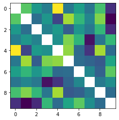
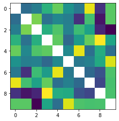
可视化


def visualize_digit_embedding(digit_embed):
  cossim_mat = []
  for i in range(10):
    cossim = torch.cosine_similarity(digit_embed, digit_embed[i:i+1,:]).cpu()
    cossim_mat.append(cossim)
  cossim_mat = torch.stack(cossim_mat)
  cossim_mat_nodiag = cossim_mat + torch.diag_embed(torch.nan * torch.ones(10))
  plt.imshow(cossim_mat_nodiag)
  plt.show()
  return cossim_mat

cossim_mat = visualize_digit_embedding(score_model.module.cond_embed.weight.data)

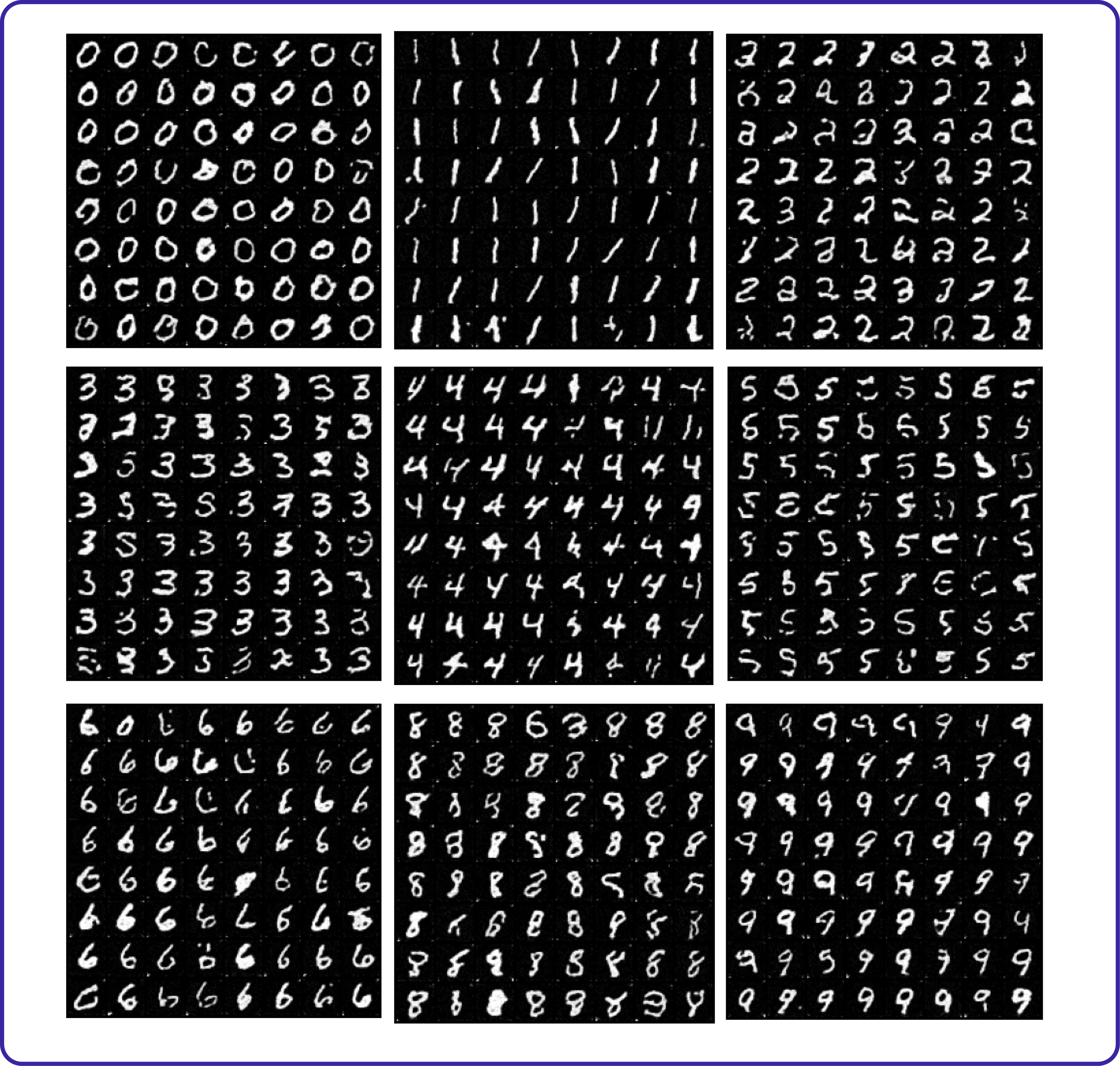
def save_samples_cond(score_model, suffix):
  score_model.eval()
  for digit in range(10):
    ## Generate samples using the specified sampler.
    sample_batch_size = 64 #@param {'type':'integer'}
    num_steps = 500 #@param {'type':'integer'}
    sampler = Euler_Maruyama_sampler #@param ['Euler_Maruyama_sampler', 'pc_sampler', 'ode_sampler'] {'type': 'raw'}
    # score_model.eval()
    ## Generate samples using the specified sampler.
    samples = sampler(score_model, 
            marginal_prob_std_fn,
            diffusion_coeff_fn, 
            sample_batch_size, 
            num_steps=num_steps,
            device=device,
            y=digit*torch.ones(sample_batch_size, dtype=torch.long))

        ## Sample visualization.
    samples = samples.clamp(0.0, 1.0)
    sample_grid = make_grid(samples, nrow=int(np.sqrt(sample_batch_size)))
    sample_np = sample_grid.permute(1, 2, 0).cpu().numpy()
    plt.imsave(f"condition_diffusion{suffix}_digit%d.png"%digit, sample_np,)
    plt.figure(figsize=(6,6))
    plt.axis('off')
    plt.imshow(sample_np, vmin=0., vmax=1.)
    plt.show()
save_samples_cond(score_model,"_res") # model with res connection

隐空间扩散

与其在像素空间中扩散（即破坏并去噪每个图像的像素），我们可以尝试在某种潜在空间中进行扩散。
这有几个优点。一个明显的优点是速度：在进行正向/逆向扩散之前压缩图像，可以使生成和训练的速度更快。另一个优点是，如果仔细选择，潜在空间可能是一个更自然或更易于解释的空间来处理图像。例如，给定一组头部的图片，可能某个潜在的方向对应于头部的方向。
如果我们对选择哪个潜在空间没有任何先验的偏好，我们可以直接使用自编码器来解决问题，希望它能找到合适的东西。
在本节中，我们将使用自编码器将MNIST图像压缩到更小的规模，并将其与我们的扩散管道的其余部分结合起来。

自编码器

自编码器首先将图像“编码”成某种潜在表示，然后从该潜在表示“解码”图像。

class AutoEncoder(nn.Module):
  """A time-dependent score-based model built upon U-Net architecture."""

  def __init__(self, channels=[4, 8, 32],):
    """Initialize a time-dependent score-based network.
    Args:
      channels: The number of channels for feature maps of each resolution.
      embed_dim: The dimensionality of Gaussian random feature embeddings.
    """
    super().__init__()
    # Gaussian random feature embedding layer for time
    # Encoding layers where the resolution decreases
    self.encoder = nn.Sequential(nn.Conv2d(1, channels[0], 3, stride=1, bias=True),
                   nn.BatchNorm2d(channels[0]),
                   nn.SiLU(),
                   nn.Conv2d(channels[0], channels[1], 3, stride=2, bias=True),
                   nn.BatchNorm2d(channels[1]),
                   nn.SiLU(),
                   nn.Conv2d(channels[1], channels[2], 3, stride=1, bias=True),
                   nn.BatchNorm2d(channels[2]),
                   ) #nn.SiLU(),
    self.decoder = nn.Sequential(nn.ConvTranspose2d(channels[2], channels[1], 3, stride=1, bias=True),
                   nn.BatchNorm2d(channels[1]),
                   nn.SiLU(),
                   nn.ConvTranspose2d(channels[1], channels[0], 3, stride=2, bias=True, output_padding=1),
                   nn.BatchNorm2d(channels[0]),
                   nn.SiLU(),
                   nn.ConvTranspose2d(channels[0], 1, 3, stride=1, bias=True),
                   nn.Sigmoid(),)
  
  def forward(self, x):
    encoded = self.encoder(x)
    output = self.decoder(encoded)
    return output

x_tmp = torch.randn(1,1,28,28)
print(AutoEncoder()(x_tmp).shape)
assert AutoEncoder()(x_tmp).shape == x_tmp.shape, "Check conv layer spec! the autoencoder input output shape not align"

用感知损失训练自动编码器

from lpips import LPIPS
device = 'cuda' #@param ['cuda', 'cpu'] {'type':'string'}
# Define the loss function, MSE and LPIPS 
lpips = LPIPS(net="squeeze").cuda()
loss_fn_ae = lambda x,xhat: \
    nn.functional.mse_loss(x, xhat) + \
    lpips(x.repeat(1,3,1,1), x_hat.repeat(1,3,1,1)).mean()

ae_model = AutoEncoder([4, 4, 4]).cuda()
n_epochs =   50  #@param {'type':'integer'}
## size of a mini-batch
batch_size =  2048   #@param {'type':'integer'}
## learning rate
lr=10e-4 #@param {'type':'number'}

dataset = MNIST('.', train=True, transform=transforms.ToTensor(), download=True)
data_loader = DataLoader(dataset, batch_size=batch_size, shuffle=True, num_workers=0)

optimizer = Adam(ae_model.parameters(), lr=lr)
tqdm_epoch = trange(n_epochs)
for epoch in tqdm_epoch:
  avg_loss = 0.
  num_items = 0
  for x, y in data_loader:
    x = x.to(device)    
    z = ae_model.encoder(x)
    x_hat = ae_model.decoder(z)
    loss = loss_fn_ae(x, x_hat) #loss_fn_cond(score_model, x, y, marginal_prob_std_fn)
    optimizer.zero_grad()
    loss.backward()    
    optimizer.step()
    avg_loss += loss.item() * x.shape[0]
    num_items += x.shape[0]
  print('{} Average Loss: {:5f}'.format(epoch, avg_loss / num_items))
  # Print the averaged training loss so far.
  tqdm_epoch.set_description('Average Loss: {:5f}'.format(avg_loss / num_items))
  # Update the checkpoint after each epoch of training.
  torch.save(ae_model.state_dict(), 'ckpt_ae.pth')

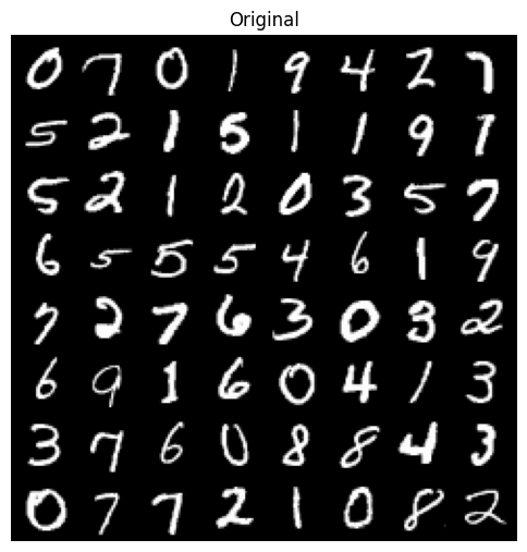
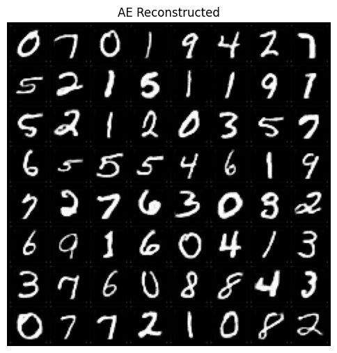
可视化训练过的自动编码器

下面的单元格用于可视化结果。自动编码器的输出应该与原始图像几乎一模一样。

#@title Visualize trained autoencoder
ae_model.eval()
x, y = next(iter(data_loader))
x_hat = ae_model(x.to(device)).cpu()
plt.figure(figsize=(6,6.5))
plt.axis('off')
plt.imshow(make_grid(x[:64,:,:,:].cpu()).permute([1,2,0]), vmin=0., vmax=1.)
plt.title("Original")
plt.show()

plt.figure(figsize=(6,6.5))
plt.axis('off')
plt.imshow(make_grid(x_hat[:64,:,:,:].cpu()).permute([1,2,0]), vmin=0., vmax=1.)
plt.title("AE Reconstructed")
plt.show()

创建潜在状态数据集

让我们使用自动编码器将MNIST图像转换为潜在空间表示。我们将使用这些压缩后的图像来训练我们的扩散生成模型。

batch_size = 4096
dataset = MNIST('.', train=True, transform=transforms.ToTensor(), download=True)
data_loader = DataLoader(dataset, batch_size=batch_size, shuffle=False, num_workers=4)
ae_model.requires_grad_(False)
ae_model.eval()
zs = []
ys = []
for x, y in tqdm(data_loader):
  z = ae_model.encoder(x.to(device)).cpu()
  zs.append(z)
  ys.append(y)

zdata = torch.cat(zs, )
ydata = torch.cat(ys, )

print(zdata.shape)
print(ydata.shape)
print(zdata.mean(), zdata.var())

from torch.utils.data import TensorDataset
latent_dataset = TensorDataset(zdata, ydata)

用于潜变量的变压器UNet模型

有一个U-Net（包括自注意力/交叉注意力），类似于我们之前定义的那种，但这次它处理的是压缩图像而不是全尺寸图像。

class Latent_UNet_Tranformer(nn.Module):
  """A time-dependent score-based model built upon U-Net architecture."""

  def __init__(self, marginal_prob_std, channels=[4, 64, 128, 256], embed_dim=256, 
               text_dim=256, nClass=10):
    """Initialize a time-dependent score-based network.

    Args:
      marginal_prob_std: A function that takes time t and gives the standard
        deviation of the perturbation kernel p_{0t}(x(t) | x(0)).
      channels: The number of channels for feature maps of each resolution.
      embed_dim: The dimensionality of Gaussian random feature embeddings.
    """
    super().__init__()
    # Gaussian random feature embedding layer for time
    self.time_embed = nn.Sequential(
        GaussianFourierProjection(embed_dim=embed_dim),
        nn.Linear(embed_dim, embed_dim))
    # Encoding layers where the resolution decreases
    self.conv1 = nn.Conv2d(channels[0], channels[1], 3, stride=1, bias=False)
    self.dense1 = Dense(embed_dim, channels[1])
    self.gnorm1 = nn.GroupNorm(4, num_channels=channels[1])
    self.conv2 = nn.Conv2d(channels[1], channels[2], 3, stride=2, bias=False)
    self.dense2 = Dense(embed_dim, channels[2])
    self.gnorm2 = nn.GroupNorm(4, num_channels=channels[2])
    self.attn2 = SpatialTransformer(channels[2], text_dim)
    self.conv3 = nn.Conv2d(channels[2], channels[3], 3, stride=2, bias=False)
    self.dense3 = Dense(embed_dim, channels[3])
    self.gnorm3 = nn.GroupNorm(4, num_channels=channels[3])   
    self.attn3 = SpatialTransformer(channels[3], text_dim) 
    
    self.tconv3 = nn.ConvTranspose2d(channels[3], channels[2], 3, stride=2, bias=False, )    
    self.dense6 = Dense(embed_dim, channels[2])
    self.tgnorm3 = nn.GroupNorm(4, num_channels=channels[2])
    self.attn6 = SpatialTransformer(channels[2], text_dim)
    self.tconv2 = nn.ConvTranspose2d(channels[2], channels[1], 3, stride=2, bias=False, output_padding=1)     # + channels[2]
    self.dense7 = Dense(embed_dim, channels[1])
    self.tgnorm2 = nn.GroupNorm(4, num_channels=channels[1])
    self.tconv1 = nn.ConvTranspose2d(channels[1], channels[0], 3, stride=1) # + channels[1]
    
    # The swish activation function
    self.act = nn.SiLU() # lambda x: x * torch.sigmoid(x)
    self.marginal_prob_std = marginal_prob_std
    self.cond_embed = nn.Embedding(nClass, text_dim)
  
  def forward(self, x, t, y=None): 
    # Obtain the Gaussian random feature embedding for t   
    embed = self.act(self.time_embed(t))    
    y_embed = self.cond_embed(y).unsqueeze(1)
    # Encoding path
    ## Incorporate information from t
    h1 = self.conv1(x) + self.dense1(embed)
    ## Group normalization
    h1 = self.act(self.gnorm1(h1))
    h2 = self.conv2(h1) + self.dense2(embed)
    h2 = self.act(self.gnorm2(h2))
    h2 = self.attn2(h2, y_embed)
    h3 = self.conv3(h2) + self.dense3(embed)
    h3 = self.act(self.gnorm3(h3))
    h3 = self.attn3(h3, y_embed)

    # Decoding path
    ## Skip connection from the encoding path
    h = self.tconv3(h3) + self.dense6(embed)
    h = self.act(self.tgnorm3(h))
    h = self.attn6(h, y_embed)
    h = self.tconv2(h + h2)
    h += self.dense7(embed)
    h = self.act(self.tgnorm2(h))
    h = self.tconv1(h + h1)

    # Normalize output
    h = h / self.marginal_prob_std(t)[:, None, None, None]
    return h

训练隐扩散模型

最后，我们将所有内容整合在一起，将我们的潜在空间表示与我们先进的U-Net结合起来学习评分函数。（这可能实际上效果不是很好…但至少你可以理解，有了这么多的活动部件，这成了一个复杂的工程问题。）
运行下面的单元来训练我们的潜在扩散模型！

#@title Training Latent diffusion model

continue_training = False #@param {type:"boolean"}
if not continue_training:
  print("initilize new score model...")
  latent_score_model = torch.nn.DataParallel(
      Latent_UNet_Tranformer(marginal_prob_std=marginal_prob_std_fn,
                  channels=[4, 16, 32, 64], ))
  latent_score_model = latent_score_model.to(device)


n_epochs =   250 #@param {'type':'integer'}
## size of a mini-batch
batch_size =  1024 #@param {'type':'integer'}
## learning rate
lr=1e-4 #@param {'type':'number'}

latent_data_loader = DataLoader(latent_dataset, batch_size=batch_size, shuffle=True, )
latent_score_model.train()
optimizer = Adam(latent_score_model.parameters(), lr=lr)
scheduler = LambdaLR(optimizer, lr_lambda=lambda epoch: max(0.5, 0.995 ** epoch))
tqdm_epoch = trange(n_epochs)
for epoch in tqdm_epoch:
  avg_loss = 0.
  num_items = 0
  for z, y in latent_data_loader:
    z = z.to(device)    
    loss = loss_fn_cond(latent_score_model, z, y, marginal_prob_std_fn)
    optimizer.zero_grad()
    loss.backward()    
    optimizer.step()
    avg_loss += loss.item() * z.shape[0]
    num_items += z.shape[0]
  scheduler.step()
  lr_current = scheduler.get_last_lr()[0]
  print('{} Average Loss: {:5f} lr {:.1e}'.format(epoch, avg_loss / num_items, lr_current))
  # Print the averaged training loss so far.
  tqdm_epoch.set_description('Average Loss: {:5f}'.format(avg_loss / num_items))
  # Update the checkpoint after each epoch of training.
  torch.save(latent_score_model.state_dict(), 'ckpt_latent_diff_transformer.pth')

可视化

digit = 4 #@param {'type':'integer'}
sample_batch_size = 64 #@param {'type':'integer'}
num_steps = 500 #@param {'type':'integer'}
sampler = Euler_Maruyama_sampler #@param ['Euler_Maruyama_sampler', 'pc_sampler', 'ode_sampler'] {'type': 'raw'}
latent_score_model.eval()
## Generate samples using the specified sampler.
samples_z = sampler(latent_score_model, 
        marginal_prob_std_fn,
        diffusion_coeff_fn, 
        sample_batch_size, 
        num_steps=num_steps,
        device=device,
        x_shape=(4,10,10),
        y=digit*torch.ones(sample_batch_size, dtype=torch.long))

## Sample visualization.
decoder_samples = ae_model.decoder(samples_z).clamp(0.0, 1.0)
sample_grid = make_grid(decoder_samples, nrow=int(np.sqrt(sample_batch_size)))
%matplotlib inline
import matplotlib.pyplot as plt

plt.figure(figsize=(6,6))
plt.axis('off')
plt.imshow(sample_grid.permute(1, 2, 0).cpu(), vmin=0., vmax=1.)
plt.show()

# play with architecturs
latent_score_model = torch.nn.DataParallel(
    Latent_UNet_Tranformer(marginal_prob_std=marginal_prob_std_fn,
                channels=[4, 16, 32, 64], ))
latent_score_model = latent_score_model.to(device)

train_diffusion_model(latent_dataset, score_model,
                      n_epochs =   100,
                      batch_size =  1024,
                      lr=10e-4,
                      model_name="transformer_latent")

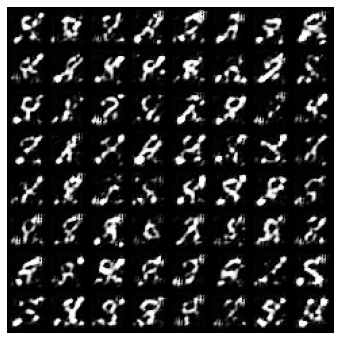
在下面，我们将详细检查一些样本，以研究图像生成的质量。你可能会看到一些相当奇怪的东西。

cossim_mat = visualize_digit_embedding(latent_score_model.module.cond_embed.weight.data)
digit = 8 #@param {'type':'integer'}
sample_batch_size = 64 #@param {'type':'integer'}
num_steps = 250 #@param {'type':'integer'}
sampler = Euler_Maruyama_sampler #@param ['Euler_Maruyama_sampler', 'pc_sampler', 'ode_sampler'] {'type': 'raw'}
latent_score_model.eval()
## Generate samples using the specified sampler.
samples_z = sampler(latent_score_model, 
        marginal_prob_std_fn,
        diffusion_coeff_fn, 
        sample_batch_size, 
        num_steps=num_steps,
        device=device,
        x_shape=(4,10,10),
        y=digit*torch.ones(sample_batch_size, dtype=torch.long))

## Sample visualization.
decoder_samples = ae_model.decoder(samples_z).clamp(0.0, 1.0)
sample_grid = make_grid(decoder_samples, nrow=int(np.sqrt(sample_batch_size)))
%matplotlib inline
import matplotlib.pyplot as plt

plt.figure(figsize=(6,6))
plt.axis('off')
plt.imshow(sample_grid.permute(1, 2, 0).cpu(), vmin=0., vmax=1.)
plt.show()

远洋之帆

关注

14
点赞
踩
9

收藏

觉得还不错? 一键收藏
0
评论
物理学视角讲解diffusion生成模型——隐扩散模型

https://zhuanlan.zhihu.com/p/692996885https://zhuanlan.zhihu.com/p/693255617前面两篇文章介绍了扩散过程，同时实现了1维、2维混合高斯扩散、逆扩散，通过模型预测得分函数来实现逆扩散推理。这个章节介绍工业界使用的文本生成图扩撒模型：stable diffusion。后面章节会将上述每个部分的一些内容代码实现，到最后将拥有一个运行中的类Stable-Diffusion模型。让我们从正向扩散开始。在最简单的情况下，相关的扩散方程是：K
复制链接

扫一扫