Python+OpenCV：傅里叶变换(Fourier Transform)

Python+OpenCV：傅里叶变换(Fourier Transform)

####################################################################################################
# 图像傅里叶变换(Image Fourier Transform)
def lmc_cv_image_fourier_transform():
    """
        函数功能: 图像傅里叶变换(Image Fourier Transform)。
    """

    # Fourier Transform in Numpy
    image = lmc_cv.imread('D:/99-Research/Python/Image/messi.jpg', flags=lmc_cv.IMREAD_GRAYSCALE)
    fft_image = np.fft.fft2(image)
    fft_shift_image = np.fft.fftshift(fft_image)
    magnitude_spectrum = 20 * np.log(np.abs(fft_shift_image))
    pyplot.figure('Fourier Transform in Numpy')
    pyplot.subplot(1, 2, 1)
    pyplot.imshow(image, cmap='gray')
    pyplot.title('Original Image')
    pyplot.xticks([])
    pyplot.yticks([])
    pyplot.subplot(1, 2, 2)
    pyplot.imshow(magnitude_spectrum, cmap='gray')
    pyplot.title('Magnitude Spectrum')
    pyplot.xticks([])
    pyplot.yticks([])
    pyplot.show()

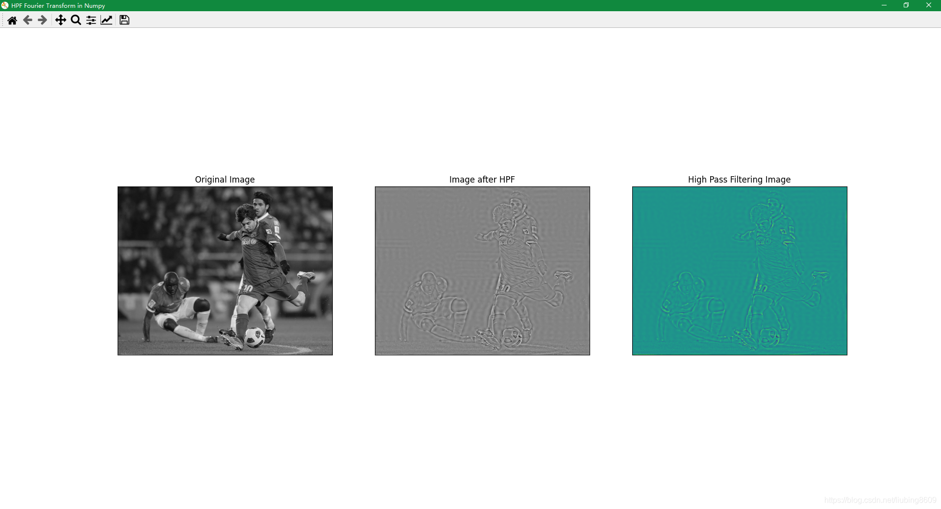
    # high pass filtering and reconstruct the image in Numpy
    rows, cols = image.shape
    crow, ccol = rows // 2, cols // 2
    fft_shift_image[crow - 30:crow + 31, ccol - 30:ccol + 31] = 0
    fft_ishift = np.fft.ifftshift(fft_shift_image)
    inverse_image_complex = np.fft.ifft2(fft_ishift)
    inverse_image_real = np.real(inverse_image_complex)
    pyplot.figure('HPF Fourier Transform in Numpy')
    pyplot.subplot(1, 3, 1)
    pyplot.imshow(image, cmap='gray')
    pyplot.title('Original Image')
    pyplot.xticks([])
    pyplot.yticks([])
    pyplot.subplot(1, 3, 2)
    pyplot.imshow(inverse_image_real, cmap='gray')
    pyplot.title('Image after HPF')
    pyplot.xticks([])
    pyplot.yticks([])
    pyplot.subplot(1, 3, 3)
    pyplot.imshow(inverse_image_real)
    pyplot.title('High Pass Filtering Image')
    pyplot.xticks([])
    pyplot.yticks([])
    pyplot.show()

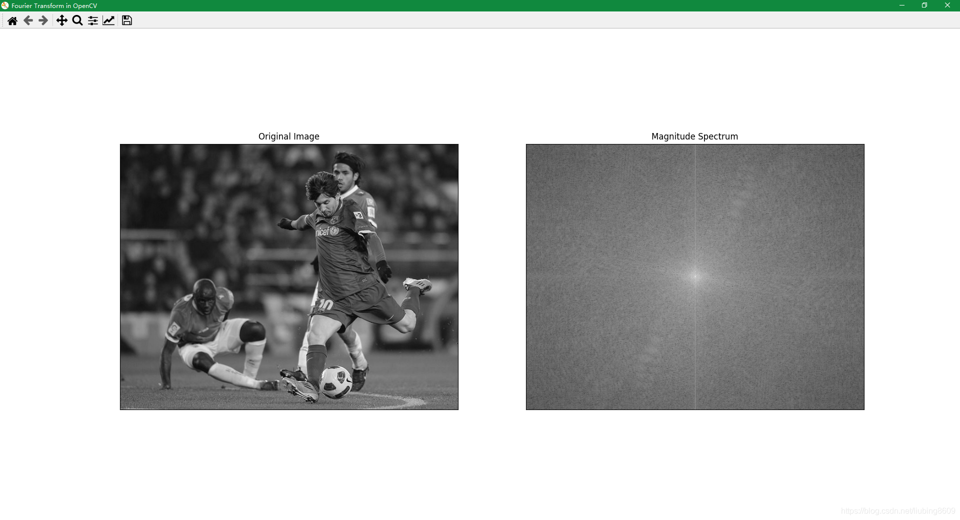
    # Fourier Transform in OpenCV
    dft_image = lmc_cv.dft(np.float32(image), flags=lmc_cv.DFT_COMPLEX_OUTPUT)
    dft_shift_image = np.fft.fftshift(dft_image)
    magnitude_spectrum = 20 * np.log(lmc_cv.magnitude(dft_shift_image[:, :, 0], dft_shift_image[:, :, 1]))
    pyplot.figure('Fourier Transform in OpenCV')
    pyplot.subplot(1, 2, 1)
    pyplot.imshow(image, cmap='gray')
    pyplot.title('Original Image')
    pyplot.xticks([])
    pyplot.yticks([])
    pyplot.subplot(1, 2, 2)
    pyplot.imshow(magnitude_spectrum, cmap='gray')
    pyplot.title('Magnitude Spectrum')
    pyplot.xticks([])
    pyplot.yticks([])
    pyplot.show()

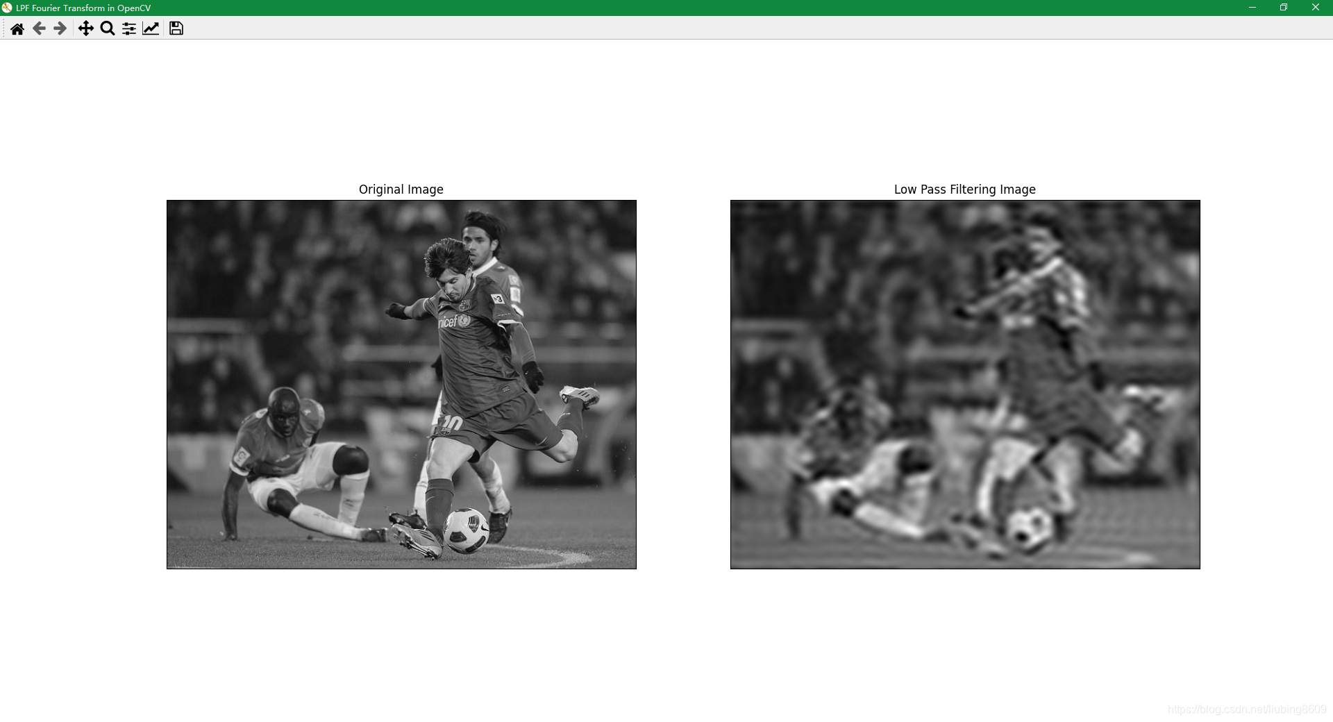
    # low pass filtering and reconstruct the image in OpenCV
    rows, cols = image.shape
    crow, ccol = rows // 2, cols // 2
    # create a mask first, center square is 1, remaining all zeros
    mask = np.zeros((rows, cols, 2), np.uint8)
    mask[crow - 30:crow + 30, ccol - 30:ccol + 30] = 1
    # apply mask and inverse DFT
    fft_shift_image = dft_shift_image * mask
    fft_ishift = np.fft.ifftshift(fft_shift_image)
    inverse_image = lmc_cv.idft(fft_ishift)
    inverse_image = lmc_cv.magnitude(inverse_image[:, :, 0], inverse_image[:, :, 1])
    pyplot.figure('LPF Fourier Transform in OpenCV')
    pyplot.subplot(1, 2, 1)
    pyplot.imshow(image, cmap='gray')
    pyplot.title('Original Image')
    pyplot.xticks([])
    pyplot.yticks([])
    pyplot.subplot(1, 2, 2)
    pyplot.imshow(inverse_image, cmap='gray')
    pyplot.title('Low Pass Filtering Image')
    pyplot.xticks([])
    pyplot.yticks([])
    pyplot.show()

    # Performance Optimization of DFT
    print("{} {}".format(rows, cols))
    nrows = lmc_cv.getOptimalDFTSize(rows)
    ncols = lmc_cv.getOptimalDFTSize(cols)
    print("{} {}".format(nrows, ncols))
    # pad zeros method 1
    new_image = np.zeros((nrows, ncols))
    new_image[:rows, :cols] = image
    # pad zeros method 2
    right = ncols - cols
    bottom = nrows - rows
    bordertype = lmc_cv.BORDER_CONSTANT  # just to avoid line breakup in PDF file
    new_image = lmc_cv.copyMakeBorder(image, 0, bottom, 0, right, bordertype, value=0)
    # calculate the DFT performance comparison of Numpy function
    number = 1000
    start_time = time.time()
    for i in range(number):
        np.fft.fft2(image)
    print(f"{number} loops, best of {(time.time() - start_time) / number} ms per loop")
    start_time = time.time()
    for i in range(number):
        np.fft.fft2(image, [nrows, ncols])
    print(f"{number} loops, best of {(time.time() - start_time) / number} ms per loop")
    # calculate the DFT performance comparison of OpenCV function
    start_time = time.time()
    for i in range(number):
        lmc_cv.dft(np.float32(image), flags=lmc_cv.DFT_COMPLEX_OUTPUT)
    print(f"{number} loops, best of {(time.time() - start_time) / number} ms per loop")
    start_time = time.time()
    for i in range(number):
        lmc_cv.dft(np.float32(new_image), flags=lmc_cv.DFT_COMPLEX_OUTPUT)
    print(f"{number} loops, best of {(time.time() - start_time) / number} ms per loop")

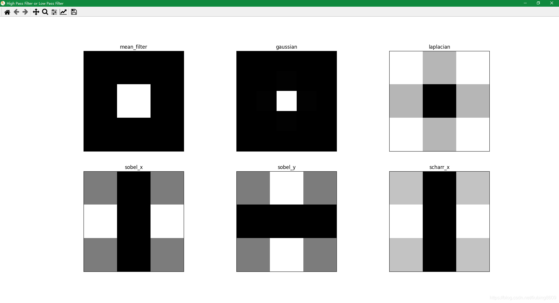
    # High Pass Filter or Low Pass Filter
    # simple averaging filter without scaling parameter
    mean_filter = np.ones((3, 3))
    # creating a gaussian filter
    x = lmc_cv.getGaussianKernel(5, 10)
    gaussian = x * x.T
    # different edge detecting filters
    # scharr in x-direction
    scharr = np.array([[-3, 0, 3],
                       [-10, 0, 10],
                       [-3, 0, 3]])
    # sobel in x direction
    sobel_x = np.array([[-1, 0, 1],
                        [-2, 0, 2],
                        [-1, 0, 1]])
    # sobel in y direction
    sobel_y = np.array([[-1, -2, -1],
                        [0, 0, 0],
                        [1, 2, 1]])
    # laplacian
    laplacian = np.array([[0, 1, 0],
                          [1, -4, 1],
                          [0, 1, 0]])
    filters = [mean_filter, gaussian, laplacian, sobel_x, sobel_y, scharr]
    filter_name = ['mean_filter', 'gaussian', 'laplacian', 'sobel_x', 'sobel_y', 'scharr_x']
    fft_filters = [np.fft.fft2(x) for x in filters]
    fft_shift = [np.fft.fftshift(y) for y in fft_filters]
    magnitude_spectrum = [20 * np.log(np.abs(z) + 1.00) for z in fft_shift]
    pyplot.figure('High Pass Filter or Low Pass Filter')
    for i in range(6):
        pyplot.subplot(2, 3, i + 1)
        pyplot.imshow(magnitude_spectrum[i], cmap='gray')
        pyplot.title(filter_name[i])
        pyplot.xticks([])
        pyplot.yticks([])
    pyplot.show()

    # 根据用户输入保存图像
    if ord("q") == (lmc_cv.waitKey(0) & 0xFF):
        # 销毁窗口
        pyplot.close('all')
    return

 

 

Performance Optimization of DFT

581 739
600 750

calculate the DFT performance comparison of Numpy function:
1000 loops, best of 0.057367880821228026 ms per loop
1000 loops, best of 0.022089494943618775 ms per loop

calculate the DFT performance comparison of OpenCV function:
1000 loops, best of 0.010666451215744019 ms per loop
1000 loops, best of 0.005198104381561279 ms per loop