【手把手教你】搭建神经网络（图像分割）

最新推荐文章于 2023-10-16 09:26:27 发布

羽峰码字

最新推荐文章于 2023-10-16 09:26:27 发布

阅读量4.8k

点赞数 11

分类专栏：图像分割深度学习机器学习文章标签：深度学习神经网络图像分割

本文链接：https://blog.csdn.net/m0_37940804/article/details/116610805

版权

深度学习同时被 3 个专栏收录

22 篇文章 21 订阅

订阅专栏

机器学习

6 篇文章 1 订阅

订阅专栏

图像分割

2 篇文章 1 订阅

订阅专栏

大家好，我是羽峰，今天要给大家分享的是一个图像分割网络，文章会把整个代码进行分割讲解，完整看完，相信你一定会有所收获。

1. 认识图像分割

2. 基于深度学习的分割

1. Oxford-IIIT Pet 数据集介绍

2. 下载 Oxford-IIIT Pets 数据集

3. 定义模型

4. 训练模型

5. 做出预测

1. 认识图像分割

图像分割是指根据灰度、彩色、空间纹理、几何形状等特征把图像划分成若干个互不相交的区域，使得这些特征在同一区域内表现出一致性或相似性，而在不同区域间表现出明显的不同。简单的说就是在一副图像中，把目标从背景中分离出来。对于灰度图像来说，区域内部的像素一般具有灰度相似性，而在区域的边界上一般具有灰度不连续性。

传统方法有：

1. 基于阈值的分割方法

2. 基于区域的图像分割方法

3. 基于边缘检测的分割方法

4. 基于小波小波变换的图像分割方法

5. 基于遗传算法的图像分割

6. 基于主动轮廓模型的分割方法

2. 基于深度学习的分割

1. Oxford-IIIT Pet 数据集介绍

本教程将使用的数据集是 Oxford-IIIT Pet 数据集，由 Parkhi et al. 创建。该数据集由图像、图像所对应的标签、以及对像素逐一标记的掩码组成。掩码其实就是给每个像素的标签。每个像素分别属于以下三个类别中的一个：

类别 1：像素是宠物的一部分。
类别 2：像素是宠物的轮廓。
类别 3：以上都不是/外围像素。

pip install -q git+https://github.com/tensorflow/examples.git

import tensorflow as tf
from tensorflow_examples.models.pix2pix import pix2pix

import tensorflow_datasets as tfds
tfds.disable_progress_bar()

from IPython.display import clear_output
import matplotlib.pyplot as plt

2. 下载 Oxford-IIIT Pets 数据集

这个数据集已经集成在 Tensorflow datasets 中，只需下载即可。图像分割掩码在版本 3.0.0 中才被加入，因此我们特别选用这个版本。

dataset, info = tfds.load('oxford_iiit_pet:3.*.*', with_info=True)

下面的代码进行了一个简单的图像翻转扩充。然后，将图像标准化到 [0,1]。最后，如上文提到的，像素点在图像分割掩码中被标记为 {1, 2, 3} 中的一个。为了方便起见，我们将分割掩码都减 1，得到了以下的标签：{0, 1, 2}。

def normalize(input_image, input_mask):
  input_image = tf.cast(input_image, tf.float32) / 255.0
  input_mask -= 1
  return input_image, input_mask

@tf.function
def load_image_train(datapoint):
  input_image = tf.image.resize(datapoint['image'], (128, 128))
  input_mask = tf.image.resize(datapoint['segmentation_mask'], (128, 128))

  if tf.random.uniform(()) > 0.5:
    input_image = tf.image.flip_left_right(input_image)
    input_mask = tf.image.flip_left_right(input_mask)

  input_image, input_mask = normalize(input_image, input_mask)

  return input_image, input_mask

def load_image_test(datapoint):
  input_image = tf.image.resize(datapoint['image'], (128, 128))
  input_mask = tf.image.resize(datapoint['segmentation_mask'], (128, 128))

  input_image, input_mask = normalize(input_image, input_mask)

  return input_image, input_mask

数据集已经包含了所需的测试集和训练集划分，所以我们也延续使用相同的划分。

TRAIN_LENGTH = info.splits['train'].num_examples
BATCH_SIZE = 64
BUFFER_SIZE = 1000
STEPS_PER_EPOCH = TRAIN_LENGTH // BATCH_SIZE

train = dataset['train'].map(load_image_train, num_parallel_calls=tf.data.experimental.AUTOTUNE)
test = dataset['test'].map(load_image_test)

train_dataset = train.cache().shuffle(BUFFER_SIZE).batch(BATCH_SIZE).repeat()
train_dataset = train_dataset.prefetch(buffer_size=tf.data.experimental.AUTOTUNE)
test_dataset = test.batch(BATCH_SIZE)

我们来看一下数据集中的一例图像以及它所对应的掩码。

def display(display_list):
  plt.figure(figsize=(15, 15))

  title = ['Input Image', 'True Mask', 'Predicted Mask']

  for i in range(len(display_list)):
    plt.subplot(1, len(display_list), i+1)
    plt.title(title[i])
    plt.imshow(tf.keras.preprocessing.image.array_to_img(display_list[i]))
    plt.axis('off')
  plt.show()

for image, mask in train.take(1):
  sample_image, sample_mask = image, mask
display([sample_image, sample_mask])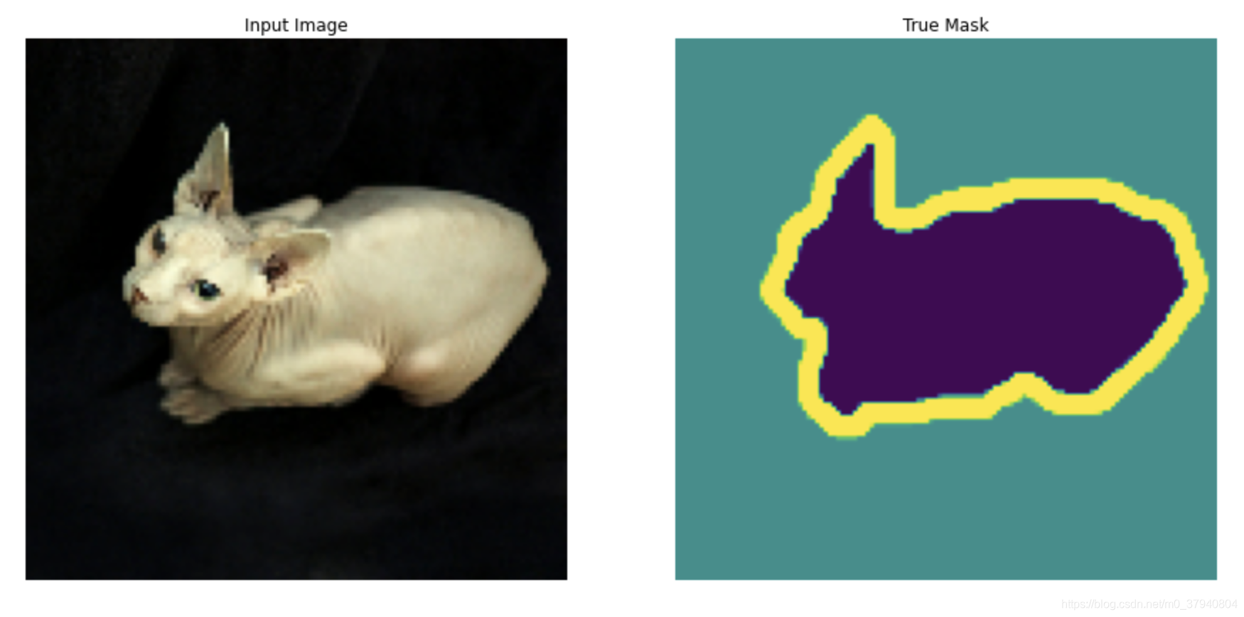

3. 定义模型

这里用到的模型是一个改版的 U-Net。U-Net 由一个编码器（下采样器（downsampler））和一个解码器（上采样器（upsampler））组成。为了学习到鲁棒的特征，同时减少可训练参数的数量，这里可以使用一个预训练模型作为编码器。因此，这项任务中的编码器将使用一个预训练的 MobileNetV2 模型，它的中间输出值将被使用。解码器将使用在 TensorFlow Examples 中的 Pix2pix tutorial 里实施过的升频取样模块。

输出信道数量为 3 是因为每个像素有三种可能的标签。把这想象成一个多类别分类，每个像素都将被分到三个类别当中。

OUTPUT_CHANNELS = 3

如之前提到的，编码器是一个预训练的 MobileNetV2 模型，它在 tf.keras.applications 中已被准备好并可以直接使用。编码器中包含模型中间层的一些特定输出。注意编码器在模型的训练过程中是不会被训练的。

base_model = tf.keras.applications.MobileNetV2(input_shape=[128, 128, 3], include_top=False)

# 使用这些层的激活设置
layer_names = [
    'block_1_expand_relu',   # 64x64
    'block_3_expand_relu',   # 32x32
    'block_6_expand_relu',   # 16x16
    'block_13_expand_relu',  # 8x8
    'block_16_project',      # 4x4
]
layers = [base_model.get_layer(name).output for name in layer_names]

# 创建特征提取模型
down_stack = tf.keras.Model(inputs=base_model.input, outputs=layers)

down_stack.trainable = False

Downloading data from https://storage.googleapis.com/tensorflow/kerasapplications/mobilenet_v2/mobilenet_v2_weights_tf_dim_ordering_tf_kernels_1.0_128_no_top.h5
9412608/9406464 [==============================] - 0s 0us/step

解码器/升频取样器是简单的一系列升频取样模块，在 TensorFlow examples 中曾被实施过。

up_stack = [
    pix2pix.upsample(512, 3),  # 4x4 -> 8x8
    pix2pix.upsample(256, 3),  # 8x8 -> 16x16
    pix2pix.upsample(128, 3),  # 16x16 -> 32x32
    pix2pix.upsample(64, 3),   # 32x32 -> 64x64
]

def unet_model(output_channels):
  inputs = tf.keras.layers.Input(shape=[128, 128, 3])
  x = inputs

  # 在模型中降频取样
  skips = down_stack(x)
  x = skips[-1]
  skips = reversed(skips[:-1])

  # 升频取样然后建立跳跃连接
  for up, skip in zip(up_stack, skips):
    x = up(x)
    concat = tf.keras.layers.Concatenate()
    x = concat([x, skip])

  # 这是模型的最后一层
  last = tf.keras.layers.Conv2DTranspose(
      output_channels, 3, strides=2,
      padding='same')  #64x64 -> 128x128

  x = last(x)

  return tf.keras.Model(inputs=inputs, outputs=x)

4. 训练模型

现在，要做的只剩下编译和训练模型了。这里用到的损失函数是 losses.sparse_categorical_crossentropy。使用这个损失函数是因为神经网络试图给每一个像素分配一个标签，和多类别预测是一样的。在正确的分割掩码中，每个像素点的值是 {0,1,2} 中的一个。同时神经网络也输出三个信道。本质上，每个信道都在尝试学习预测一个类别，而 losses.sparse_categorical_crossentropy 正是这一情形下推荐使用的损失函数。根据神经网络的输出值，分配给每个像素的标签为输出值最高的信道所表示的那一类。这就是 create_mask 函数所做的工作。

model = unet_model(OUTPUT_CHANNELS)
model.compile(optimizer='adam',
              loss=tf.keras.losses.SparseCategoricalCrossentropy(from_logits=True),
              metrics=['accuracy'])

我们试着运行一下模型，看看它在训练之前给出的预测值。

def create_mask(pred_mask):
  pred_mask = tf.argmax(pred_mask, axis=-1)
  pred_mask = pred_mask[..., tf.newaxis]
  return pred_mask[0]

def show_predictions(dataset=None, num=1):
  if dataset:
    for image, mask in dataset.take(num):
      pred_mask = model.predict(image)
      display([image[0], mask[0], create_mask(pred_mask)])
  else:
    display([sample_image, sample_mask,
             create_mask(model.predict(sample_image[tf.newaxis, ...]))])

show_predictions()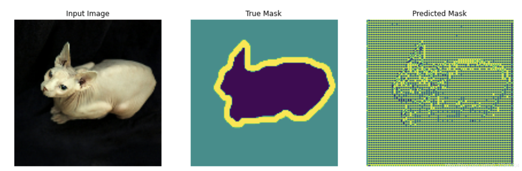

我们来观察模型是怎样随着训练而改善的。为达成这一目的，下面将定义一个 callback 函数。

class DisplayCallback(tf.keras.callbacks.Callback):
  def on_epoch_end(self, epoch, logs=None):
    clear_output(wait=True)
    show_predictions()
    print ('\nSample Prediction after epoch {}\n'.format(epoch+1))

EPOCHS = 20
VAL_SUBSPLITS = 5
VALIDATION_STEPS = info.splits['test'].num_examples//BATCH_SIZE//VAL_SUBSPLITS

model_history = model.fit(train_dataset, epochs=EPOCHS,
                          steps_per_epoch=STEPS_PER_EPOCH,
                          validation_steps=VALIDATION_STEPS,
                          validation_data=test_dataset,
                          callbacks=[DisplayCallback()])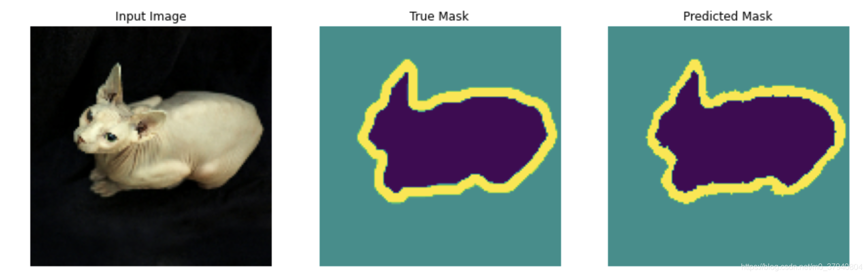

Sample Prediction after epoch 20

57/57 [==============================] - 3s 54ms/step - loss: 0.1308 - accuracy: 0.9401 - val_loss: 0.3246 - val_accuracy: 0.8903

loss = model_history.history['loss']
val_loss = model_history.history['val_loss']

epochs = range(EPOCHS)

plt.figure()
plt.plot(epochs, loss, 'r', label='Training loss')
plt.plot(epochs, val_loss, 'bo', label='Validation loss')
plt.title('Training and Validation Loss')
plt.xlabel('Epoch')
plt.ylabel('Loss Value')
plt.ylim([0, 1])
plt.legend()
plt.show()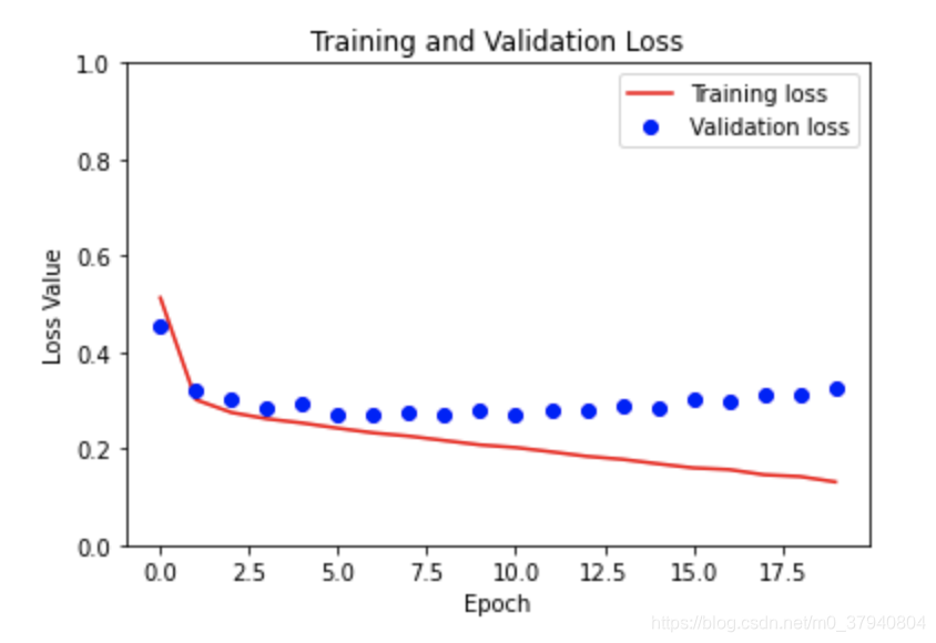

5. 做出预测

我们来做几个预测。为了节省时间，这里只使用很少的周期（epoch）数，但是你可以设置更多的数量以获得更准确的结果。

show_predictions(test_dataset, 2)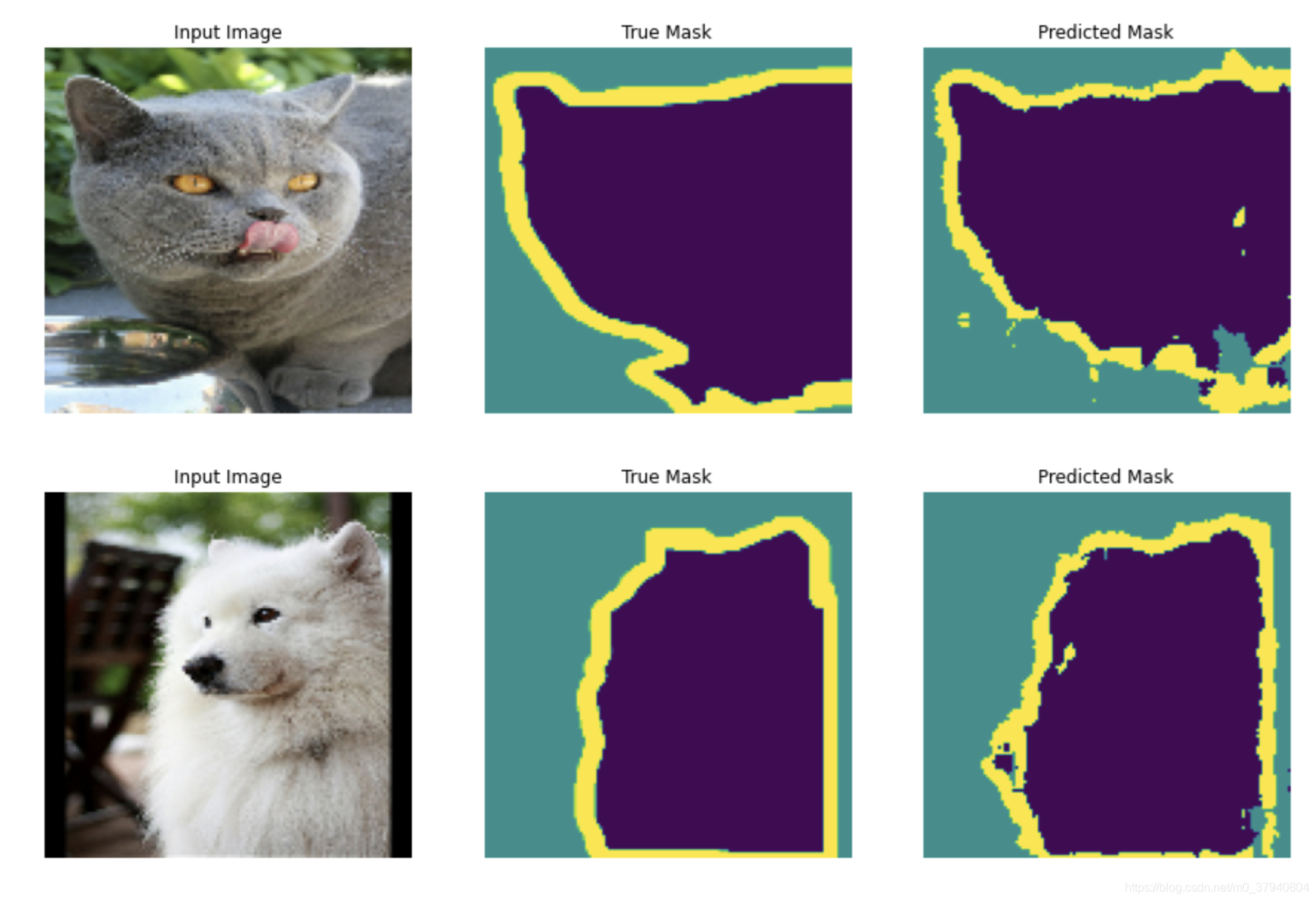

至此，今天的分享结束了，希望通过以上分享，你能学习到图像分割的基本流程，基本过程。强烈建议新手能按照上述步骤一步步实践下来，必有收获。

今天文章来源于：https://tensorflow.google.cn/tutorials/keras/classification，新入门的小伙伴可以好好看看这个网站，很基础，很适合新手。

当然，这里不得不重点推荐一下这两个网站：

https://tensorflow.google.cn/tutorials/keras/classification

https://keras.io/zh/

我是羽峰，公众号：羽峰码字，欢迎来撩

羽峰码字

关注

11
点赞
踩
64

收藏

觉得还不错? 一键收藏
打赏
18
评论
【手把手教你】搭建神经网络（图像分割）

大家好，我是羽峰，今天要给大家分享的是一个图像分割网络，文章会把整个代码进行分割讲解，完整看完，相信你一定会有所收获。目录1. 认识图像分割2.基于深度学习的分割1.Oxford-IIIT Pet 数据集介绍2. 下载 Oxford-IIIT Pets 数据集3. 定义模型4. 训练模型5. 做出预测1. 认识图像分割图像分割是指根据灰度、彩色、空间纹理、几何形状等特征把图像划分成若干个互不相交的区域，使得这些特征在同一区域内表现出一致性或相似性，而在不同区域...
复制链接

扫一扫