开始深度学习

一、生成数据集

def synthetic_data(w, b, num_examples):
    """Generate y = Xw + b + noise."""
    X = torch.normal(0, 1, (num_examples, len(w)))
    y = torch.matmul(X, w) + b
    y += torch.normal(0, 0.01, y.shape)
    return X, y.reshape((-1, 1))

此时X是一个num_examples × len(w)，均值为0，标准差为1的张量，y是num_examples × 1
的张量，再加上均值为1，标准差为0.01的噪声

true_w = torch.tensor([2, -3.4])
true_b = 4.2
features, labels = synthetic_data(true_w, true_b, 1000)

将w = ([2, -3.4]), b = 4.2输入，数据量为1000，得到原始数据集，通过matplotlib绘制出来

plt.scatter(features[:, 1].detach().numpy(), labels.detach().numpy(), 1)
plt.show()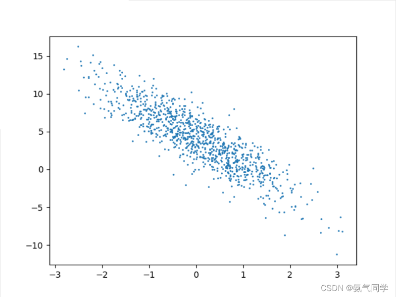

 二、读取数据集

def data_iter(batch_size, features, labels):
    """Iterate through a dataset."""
    num_examples = len(features)
    indices = list(range(num_examples))
    random.shuffle(indices)  # The examples are read at random, in no particular order
    for i in range(0, num_examples, batch_size):
        batch_indices = torch.tensor(indices[i: min(i + batch_size, num_examples)])
        yield features[batch_indices], labels[batch_indices]

• batch_size: 每个批次的样本数量
• features: 特征数据，一个特征矩阵或张量
• labels: 标签数据，对应于每个样本的目标值或类别

首先，通过 len(features) 获取样本数量，并将索引存储在 indices 列表中

使用 random.shuffle(indices) 将索引列表随机打乱，以便以随机顺序读取样本

使用 range 函数遍历样本索引，步长为 batch_size，以获取每个批次的起始索引

对于每个批次的起始索引 i，使用 torch.tensor(indices[i: min(i + batch_size, num_examples)]) 获取批次对应的索引列表，并将其转换为 PyTorch 的张量

使用获取的批次索引，通过 features[batch_indices] 和 labels[batch_indices] 获取相应的特征和标签数据，使用 yield 关键字返回每个批次的特征和标签数据 

设置批量大小为10，读取一组数据：

batch_size = 10
for X, y in data_iter(batch_size, features, labels):
    print(X, '\n', y)
    break

tensor([[-0.0696,  0.7543],
        [-0.7112,  1.1201],
        [ 0.3787, -0.1899],
        [-0.4493,  0.6387],
        [-0.0395,  1.6439],
        [ 1.6767,  0.9483],
        [-0.6776,  0.0829],
        [ 0.1027,  1.4863],
        [-0.3009,  0.3095],
        [ 0.1412,  0.5425]]) 
 tensor([[ 1.4887],
        [-1.0235],
        [ 5.6077],
        [ 1.1209],
        [-1.4830],
        [ 4.3342],
        [ 2.5570],
        [-0.6442],
        [ 2.5390],
        [ 2.6399]])

三、初始化模型参数 

w = torch.normal(0, 0.01, size=(2, 1), requires_grad=True)
b = torch.zeros(1, requires_grad=True)

 四、定义模型

def linreg(X, w, b):
    """The linear regression model."""
    return torch.matmul(X, w) + b

线性回归模型的预测值是通过将输入特征数据 X 与权重参数 w 相乘，再加上偏置参数 b 来计算的 

五、定义损失函数

def squared_loss(y_hat, y):
    """Squared loss."""
    return (y_hat - y.reshape(y_hat.shape)) ** 2 / 2

使用均方损失函数，计算预测值和真是值之间的差距 

六、定义优化算法 

def sgd(params, lr, batch_size):
    """Minibatch stochastic gradient descent."""
    with torch.no_grad():
        for param in params:
            param -= lr * param.grad / batch_size
            param.grad.zero_()

小批量随机梯度下降以最小化损失函数，对于每个需要更新的参数 param，执行以下步骤：

• 计算参数的梯度，即 param.grad。
• 将参数更新的量计算为 lr * param.grad / batch_size，其中 lr 是学习率，param.grad 是梯度，batch_size 是小批量样本的数量。
• 将参数减去更新的量，即 param -= lr * param.grad / batch_size，从而更新参数。
• 调用 param.grad.zero_() 将参数的梯度清零，以便下一次迭代计算新的梯度

七、开始训练 

 设置参数

lr = 0.03  # Learning rate
num_epochs = 3  # Number of iterations
net = linreg  # Our fancy linear model
loss = squared_loss  # 0.5 (y-y')^2

for epoch in range(num_epochs):
    for X, y in data_iter(batch_size, features, labels):
        l = loss(net(X, w, b), y)
        # Compute gradient on l with respect to [w,b]
        l.sum().backward()
        sgd([w, b], lr, batch_size)  # Update parameters using their gradient
    with torch.no_grad():
        train_l = loss(net(features, w, b), labels)
        print(f'epoch {epoch + 1}, loss {float(train_l.mean()):f}')

1. 使用 range(num_epochs) 迭代训练指定数量的 epochs。
2. 在每个 epoch 中，使用 data_iter 函数按批次遍历数据集，并获取特征 X 和标签 y。
3. 使用模型 net、权重参数 w 和偏置参数 b 来计算预测值，并计算预测值与真实值之间的损失 l。
4. 通过调用 l.sum().backward() 计算损失 l 对于参数 [w, b] 的梯度。
5. 使用 sgd([w, b], lr, batch_size) 调用小批量随机梯度下降函数，更新参数 [w, b]。
6. 在每个 epoch 结束时，使用 torch.no_grad() 上下文管理器，计算整个训练集上的损失 train_l，以评估模型的训练效果。
7. 打印当前 epoch 的序号和损失值。

通过这个训练循环，模型在每个 epoch 中都会遍历整个数据集，并使用小批量样本计算梯度和更新参数。通过不断迭代优化模型的参数，损失值将逐渐减小，模型对训练数据的拟合效果将逐渐提升。 

print(f'estimating w: {w.reshape(true_w.shape)}')
print(f'estimating b: {b}')
print(f'error in estimating w: {true_w - w.reshape(true_w.shape)}')
print(f'error in estimating b: {true_b - b}')

最后输出预测的参数值以及与真实值的误差：

estimating w: tensor([ 1.9997, -3.3996], grad_fn=<ReshapeAliasBackward0>)
estimating b: tensor([4.1995], requires_grad=True)
error in estimating w: tensor([ 0.0003, -0.0004], grad_fn=<SubBackward0>)
error in estimating b: tensor([0.0005], grad_fn=<RsubBackward1>) 

八、完整代码

import torch
import random
import matplotlib.pyplot as plt


def synthetic_data(w, b, num_examples):
    """Generate y = Xw + b + noise."""
    X = torch.normal(0, 1, (num_examples, len(w)))  # X.shape = (num_examples, len(w))
    y = torch.matmul(X, w) + b  # y.shape = (num_examples, 1)
    y += torch.normal(0, 0.01, y.shape)  # Add noise
    return X, y.reshape((-1, 1))  # y.shape = (num_examples, 1)


true_w = torch.tensor([2, -3.4])
true_b = 4.2
features, labels = synthetic_data(true_w, true_b, 1000)
plt.scatter(features[:, 1].detach().numpy(), labels.detach().numpy(), 1)
plt.show()


def data_iter(batch_size, features, labels):
    """Iterate through a dataset."""
    num_examples = len(features)
    indices = list(range(num_examples))
    random.shuffle(indices)  # The examples are read at random, in no particular order
    for i in range(0, num_examples, batch_size):
        batch_indices = torch.tensor(indices[i: min(i + batch_size, num_examples)])
        yield features[batch_indices], labels[batch_indices]


batch_size = 10
for X, y in data_iter(batch_size, features, labels):
    print(X, '\n', y)
    break
w = torch.normal(0, 0.01, size=(2, 1), requires_grad=True)
b = torch.zeros(1, requires_grad=True)


def linreg(X, w, b):
    """The linear regression model."""
    return torch.matmul(X, w) + b


def squared_loss(y_hat, y):
    """Squared loss."""
    return (y_hat - y.reshape(y_hat.shape)) ** 2 / 2


def sgd(params, lr, batch_size):
    """Minibatch stochastic gradient descent."""
    with torch.no_grad():
        for param in params:
            param -= lr * param.grad / batch_size
            param.grad.zero_()


lr = 0.03  # Learning rate
num_epochs = 3  # Number of iterations
net = linreg  # Our fancy linear model
loss = squared_loss  # 0.5 (y-y')^2

for epoch in range(num_epochs):
    for X, y in data_iter(batch_size, features, labels):
        l = loss(net(X, w, b), y)
        # Compute gradient on l with respect to [w,b]
        l.sum().backward()
        sgd([w, b], lr, batch_size)  # Update parameters using their gradient
    with torch.no_grad():
        train_l = loss(net(features, w, b), labels)
        print(f'epoch {epoch + 1}, loss {float(train_l.mean()):f}')


print(f'estimating w: {w.reshape(true_w.shape)}')
print(f'estimating b: {b}')
print(f'error in estimating w: {true_w - w.reshape(true_w.shape)}')
print(f'error in estimating b: {true_b - b}')