


1写在前面
好久没更了,实在是太忙了,值班真的是根本不不睡觉啊,一忙一整天,忙到怀疑人生。😭
最近看到比较🔥的就是ggkegg包,感觉使用起来还是有一定难度的。🫠
和大家分享一下使用教程吧,还有一些小坑。💪
2用到的包
rm(list = ls())
library(ggkegg)
library(ggfx)
library(ggraph)
library(igraph)
library(clusterProfiler)
library(dplyr)
library(tidygraph)
3小试牛刀
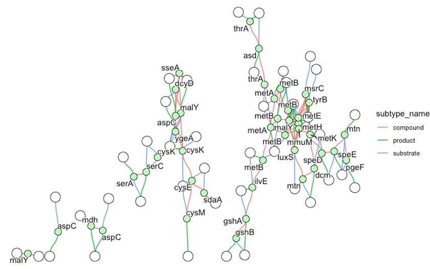
首先以eco00270为例,获取后转换路径和eco标识符,删除无连接节点并返回igraph对象。🤪
g <- ggkegg(pid="eco00270",
            convert_org = c("pathway","eco"),
            delete_zero_degree = T,
            return_igraph = T)

gg <- ggraph(g, layout="stress")
gg$data$type  %>%  unique()

gg + geom_edge_diagonal(
  aes(color=subtype_name,
      filter=type!="maplink"))+
  geom_node_point(
  aes(filter= !type%in%c("map","compound")),
    fill=gg$data[!gg$data$type%in%c("map","compound"),]$bgcolor,
    color="black",
    shape=21, size=4
  )+
  geom_node_point(
    aes(filter= !type%in%c("map","gene")),
    fill=gg$data[!gg$data$type%in%c("map","gene"),]$bgcolor,
    color="black",
    shape=21, size=6
  )+
  geom_node_text(
    aes(label=converted_name,
        filter=type=="gene"),
    repel=T,
    bg.colour="white")+
  theme_void()
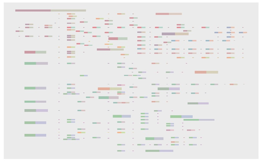
4改变nodes颜色
颜狗必备技能,修改配色。😘
g <- pathway("ko00520")
V(g)$color_one <- colorRampPalette(RColorBrewer::brewer.pal(5,"Set1"))(length(V(g)))
V(g)$color_two <- colorRampPalette(RColorBrewer::brewer.pal(5,"Set2"))(length(V(g)))

ggraph(g, x=x, y=y) +
  geom_node_rect(aes(xmin=xmin, xmax=x, fill=I(color_one)), alpha=0.5)+
  geom_node_rect(aes(xmin=x, xmax=xmax, fill=I(color_two)), alpha=0.5)+
  ggfx::with_outer_glow(geom_node_text(aes(label=name %>%
                       strsplit(":") %>%
                       sapply("[", 2) %>%
                       strsplit(" ") %>%
                       sapply("[", 1),
                     filter=type=="ortholog"),
                     size=2), colour="white", expand=1)
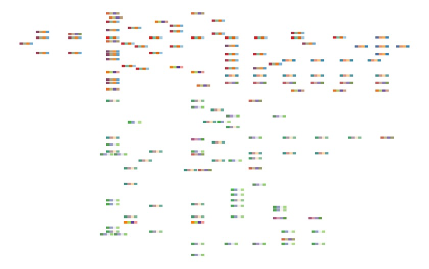
V(g)$color_one <- colorRampPalette(RColorBrewer::brewer.pal(5,"Set1"))(length(V(g)))
V(g)$color_two <- colorRampPalette(RColorBrewer::brewer.pal(5,"Set2"))(length(V(g)))
V(g)$color_three <- colorRampPalette(RColorBrewer::brewer.pal(5,"PuOr"))(length(V(g)))
V(g)$color_four <- colorRampPalette(RColorBrewer::brewer.pal(5,"Paired"))(length(V(g)))

V(g)$space <- V(g)$width/4

ggraph(g, x=x, y=y) +
  geom_node_rect(aes(xmin=xmin, xmax=xmin+space, fill=I(color_one), filter=type=="ortholog"))+
  geom_node_rect(aes(xmin=xmin+space, xmax=xmin+2*space, fill=I(color_two), filter=type=="ortholog"))+
  geom_node_rect(aes(xmin=xmin+2*space, xmax=xmin+3*space, fill=I(color_three), filter=type=="ortholog"))+
  geom_node_rect(aes(xmin=xmin+3*space, xmax=xmin+4*space, fill=I(color_four), filter=type=="ortholog"))+
  ggfx::with_outer_glow(geom_node_text(aes(label=name %>%
                                             strsplit(":") %>%
                                             sapply("[", 2) %>%
                                             strsplit(" ") %>%
                                             sapply("[", 1),
                                           filter=type=="ortholog"),
                                       size=2), colour="white", expand=1)+
  theme_void()
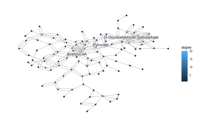
5Global maps展示
更宏观的展示结果。🤩
pathway("ko01200") %>%
    process_reaction() %>%
    activate(nodes) %>%
    mutate(x=NULL, y=NULL,
       comp=convert_id("compound")) %>%
    mutate(degree=centrality_degree(mode="all")) %>%
ggraph(layout="kk")+
    geom_node_point(aes(color=degree,
                        filter=type=="compound"))+
    geom_edge_parallel(
        color="grey",
        end_cap=circle(1,"mm"),
        start_cap=circle(1,"mm"),
        arrow=arrow(length=unit(1,"mm"),type="closed"))+
    geom_node_text(aes(label=comp,filter=degree>15),
                   repel=TRUE, bg.colour="white")+
    theme_graph()
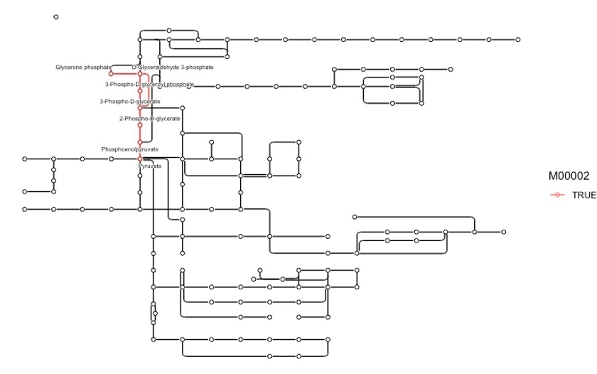
6highlight指定nodes和edges
可以使用highligh_set_edges和highlight_set_nodes函数突出你想要突出的nodes和edges。😘
pathway("ko01230") %>%
  process_line() %>%
  activate(nodes) %>%
  mutate(
    compound=convert_id("compound"),
    M00002=highlight_set_nodes(module("M00002")@reaction_components)) %>%
  activate(edges) %>%
  mutate(M00002=highlight_set_edges(module("M00002")@definition_components)) %>%
  ggraph(x=x, y=y)+
  geom_edge_link()+
  with_outer_glow(geom_edge_link(aes(color=M00002, filter=M00002)),
                  colour="pink")+
  geom_node_point(shape=21,aes(filter=type!="line"))+
  with_outer_glow(geom_node_point(shape=21, aes(filter=M00002, color=M00002)),
                  colour="pink")+
  geom_node_text(aes(label=compound, filter=M00002), repel=TRUE,
                 bg.colour="white", size=2)+
  theme_void()
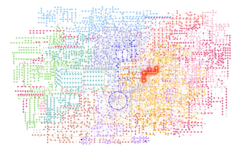
我们试着突出一下代谢相关pathway(ko01100),需要用到M00021的module。😋
g <- pathway("ko01100") %>%
  process_line() %>%
  highlight_module(module("M00021")) %>%
  mutate(compound=convert_id("compound"))

g %>% ggraph(x=x, y=y) +
  geom_node_point(size=1, aes(color=I(fgcolor),
    filter=fgcolor!="none" & type!="line"))+
  geom_edge_link(width=0.1, aes(color=I(fgcolor),
                                filter=type=="line"& fgcolor!="none"))+
  with_outer_glow(
    geom_edge_link(width=1,
                   aes(color=I(fgcolor),
                       filter=fgcolor!="none" & M00021)),
    colour="red", expand=3
  )+
  with_outer_glow(
    geom_node_point(size=2,
                   aes(color=I(fgcolor),
                       filter=fgcolor!="none" & M00021)),
    colour="red", expand=3
  )+
  theme_void()
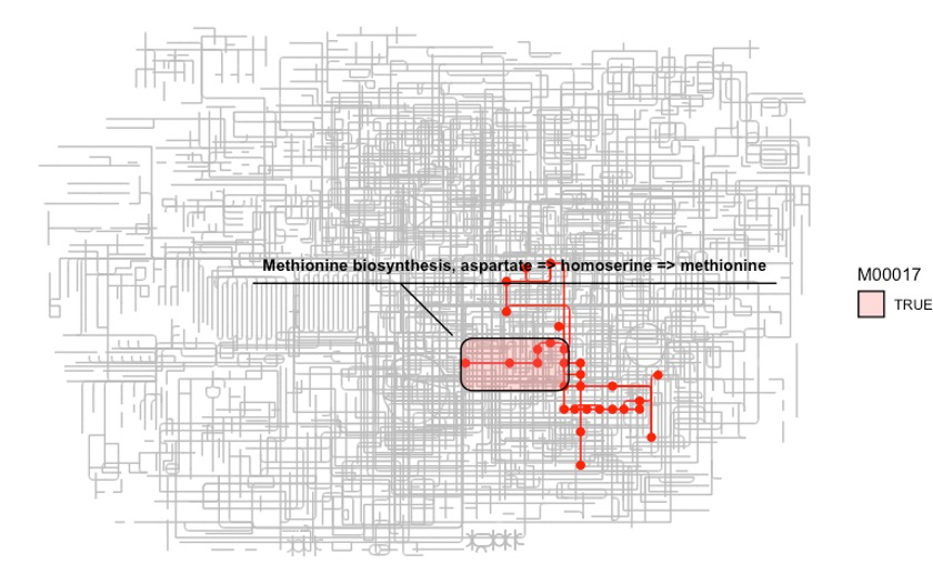
可以看到多个module涉及Cysteine和methionine的代谢,我们可以通过使用ggforce来高亮M00017。😘
list_of_modules <- c("M00021","M00338","M00609","M00017","M00034","M00035","M00368")
for (mm in list_of_modules) {
  g <- g %>% highlight_module(module(mm))
}

ggraph(g,x=x,y=y,layout="manual") +
  geom_edge_link0(width=0.5, color="grey")+
  geom_edge_link(color="red",aes(filter=M00017|M00021|M00338|M00609|M00034|M00035|M00368))+
geom_node_point(size=2, color="red",aes(filter=M00017|M00021|M00338|M00609|M00034|M00035|M00368))+
  ggforce::geom_mark_rect(aes(fill=M00017,
                              label=module("M00017")@name,
                              x=x, y=y,
                              group=M00017,
                              filter=M00017),
                          label.fill = "transparent",
                          label.fontsize = 10,
                          expand=unit(1,"mm"))+
  theme_void()
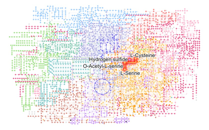
可视化一下compounds,可以用geom_node_text,ggrepel, 和shadowtext。🤪
Rg %>% ggraph(x=x, y=y) +
  geom_node_point(size=1, aes(color=I(fgcolor),
    filter=fgcolor!="none" & type!="line"))+
  geom_edge_link(width=0.1, aes(color=I(fgcolor),
                                filter=type=="line"& fgcolor!="none"))+
  with_outer_glow(
    geom_edge_link(width=1,
                   aes(color=I(fgcolor),
                       filter=fgcolor!="none" & M00021)),
    colour="red", expand=3
  )+
  with_outer_glow(
    geom_node_point(size=2,
                   aes(color=I(fgcolor),
                       filter=fgcolor!="none" & M00021)),
    colour="red", expand=3
  )+
    geom_node_text(aes(label=compound, filter=M00021),
                   repel=T, bg.colour="white", size=5)+
  theme_void()
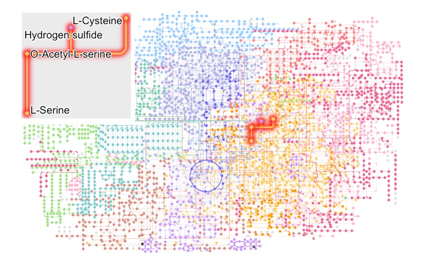
局部放大一下!~😘
annot <- g %>%  ggraph(x=x, y=y)+
  with_outer_glow(
    geom_edge_link(width=1,
                   aes(color=I(fgcolor),
                       filter=fgcolor!="none" & M00021)),
    colour="red", expand=3
  )+
  with_outer_glow(
    geom_node_point(size=2,
                    aes(color=I(fgcolor),
                        filter=fgcolor!="none" & M00021)),
    colour="red", expand=3
  )+
    geom_node_text(aes(label=compound, filter=M00021),
                   repel=TRUE, bg.colour="white", size=5)
g %>%
  ggraph(x=x, y=y) +
  geom_node_point(size=1, aes(color=I(fgcolor),
                              filter=fgcolor!="none" & type!="line"))+
  geom_edge_link(width=0.1, aes(color=I(fgcolor),
                                filter=type=="line"& fgcolor!="none"))+
  with_outer_glow(
    geom_edge_link(width=1,
                   aes(color=I(fgcolor),
                       filter=fgcolor!="none" & M00021)),
    colour="red", expand=3
  )+
  with_outer_glow(
    geom_node_point(size=2,
                    aes(color=I(fgcolor),
                        filter=fgcolor!="none" & M00021)),
    colour="red", expand=3
  )+
  annotation_custom(ggplotify::as.grob(annot),
    ymin=-1500, ymax=0, xmin=0, xmax=1500)+
  theme_void()

点个在看吧各位~ ✐.ɴɪᴄᴇ ᴅᴀʏ 〰
📍 🤩 LASSO | 不来看看怎么美化你的LASSO结果吗!?
📍 🤣 chatPDF | 别再自己读文献了!让chatGPT来帮你读吧!~
📍 🤩 WGCNA | 值得你深入学习的生信分析方法!~
📍 🤩 ComplexHeatmap | 颜狗写的高颜值热图代码!
📍 🤥 ComplexHeatmap | 你的热图注释还挤在一起看不清吗!?
📍 🤨 Google | 谷歌翻译崩了我们怎么办!?(附完美解决方案)
📍 🤩 scRNA-seq | 吐血整理的单细胞入门教程
📍 🤣 NetworkD3 | 让我们一起画个动态的桑基图吧~
📍 🤩 RColorBrewer | 再多的配色也能轻松搞定!~
📍 🧐 rms | 批量完成你的线性回归
📍 🤩 CMplot | 完美复刻Nature上的曼哈顿图
📍 🤠 Network | 高颜值动态网络可视化工具
📍 🤗 boxjitter | 完美复刻Nature上的高颜值统计图
📍 🤫 linkET | 完美解决ggcor安装失败方案(附教程)
📍 ......


本文由 mdnice 多平台发布


 2772
2772


 被折叠的 条评论
为什么被折叠?
被折叠的 条评论
为什么被折叠?
 到【灌水乐园】发言


