TorchSparse: 3D SC/SSC Acceleration on GPU

Paper:

TorchSparse: Efficient Point Cloud Inference Engine

Notation:

Mapping

 

 to get output position set:

when down-sampling, since we want to sample as many sparse input sites as possible, we slack the SSC i/o mapping condition to  p < s*b + offset, where:

==> instead of offset = 0, we check all possible offset for p to be matched to any kernel within output boundary, b_i <= B = (range(D_i) - s_i) / s_i + 1

====> u % s enforces kernel central matching after dilation

to fill out the map:

 

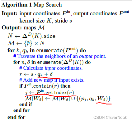
==> recall j, k will be uniquely matched via delta

==> all channels share 1 offset, i.e. the feature vector x_in * W_delta = x_out

To efficiently examine whether the possible input q_j + offset is nonzero, a common implementation is to record the coordinates of nonzero inputs with hash table. The key-value pairs are (key=input coordinates, value=input index), i.e., (key = pj ; value = j). The hash function can simply be flattening the coordinate of each dimension into an integer.

==> regarding the key-value pair, both the index and the coordinates are uniquely values, so the key-val ordering doesn't matter.

TorchSparse Schematics

place holder for figure 2

Figure 2: TorchSparse aims at accelerating Sparse Convolution, which consists of four stages: mapping, gather, matmul and scatter-accumulate. We follow two general principles that

1 memory footprint should be reduced

2 computation regularity should be increased

to optimize these four components with quantized, vectorized, row-major scatter/gather (Principle 1); adaptively batched matmul (Principle 2 ) and mapping kernel fusion (Principle 1).

Data Orchestration and Matrix Multiplication

Since the utilization ratio of matrix-vector multiplication is low on GPU, a better implementation will follow Gather-MatMul-Scatter computation flow as shown in Algorithm 2. First, all input feature vectors associated with the same weight matrix are gathered and concatenated into a contiguous matrix. Then, matrix-matrix multiplication between= feature matrix and weight matrix is conducted to obtain the partial sums. Finally, these partial sums are scattered and accumulated to the corresponding output feature vectors. 

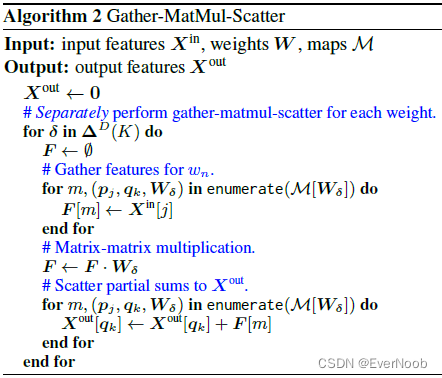
==> the locality-aware part will be explained later

compared to existing conventional conv.

with sparsity via ReLU or weight pruning ==> former suffers from dilation of sparsity 

Figure 3: SparseConv (b) does not multiply each nonzero input with all nonzero weights as conventional convolution (a) does.

compared to graph convolution:

In graph convolution, the relationship between inputs and outputs are provided in the adjacency matrix which stays constant across layers. Contrarily, sparse convolution have to search maps for every downsampling block. Furthermore, graph convolution shares same weight matrix for different neighbors, i.e. all W_off are the same. Hence, graph convolution only needs either one gather or one scatter of features: 1) first gather input features associated with the same output vertex, and then multiply them with shared weights and reduce to the output feature vector; or 2) first multiply all input features with shared weights, and then scatter-accumulate the partial sums to the corresponding output feature vector. However, sparse convolution uses different weight matrices for different kernel offset, off, and thus needs both gather and scatter during the computation. Consequently, existing SpMV/SpDMM systems for graph convolution accleration (Wang et al., 2019a; Hu et al., 2020) are not applicable to sparse convolution.

Analysis

profile of segmentation and detection shown below:

Figure 4: Data Movement and Mapping Operations constitute a significant proportion of SparseConv runtime.

Based on observations in Figure 4, we summarize two principles for SparseConv optimization which lays the foundation for our system design;

Principle I. Improve Regularity in Computation

Matrix multiplication is the core computation in SparseConv and takes up a large proportion of total execution time (20%-50%). actual matmul workloads are very non-uniform due to the irregular nature of point clouds (detailed in Figure 12, where map sizes for different weights can differ by an order of magnitude and most map sizes are small).

Figure 12: Maps on nuScenes are much smaller than on SemanticKITTI for MinkUNet model. Thus, grouping strategy on NuScenes is more aggressive (8 groups vs. 10 groups).

Principle II. Reduce Memory Footprint

On average, data movement is the largest bottleneck in SparseConvNets, which takes up 40%-50% of total runtime. This is because scatter-gather operations are bottlenecked by GPU memory bandwidth (limited) instead of computation resources (abundant). Worse still, the dataflow in Algorithm 2 completely separates scatter-gather operations for different weights. This further ruins the possibility of potential reuse in data movement, which will be detailed in Figure 9. It is also noteworthy that the large mapping latency in the Center-Point detector also stems from memory overhead: typical hashmap implementations for Algorithm 1 require multiple DRAM accesses on a hash collision, and a naive implementation of output coordinate calculation (see Appendix A==>alg.1 above) also requires multiple DRAM writes for intermediate results. Consequently, reducing memory footprint is at the heart of data movement and mapping optimization

Matrix Multiplication Optimization

Matrix multiplication is the core computation in SparseConv. Because of the irregularity of point clouds, existing implementations rely on cuDNN to perform many small matmul operations on different weights (Figure 6b), which usually do not saturate the utilization of GPUs. In order to increase the utilization, we propose to trade computation for regularity (Principle I) by grouping matmul for different weights together. We find it helpful to introduce redundant computation but group more computation in a single kernel. In Figure 12, we collect the real workload for MinkUNet (Choy et al., 2019) on SemanticKITTI (Behley et al., 2019) and analyze the efficiency of matmul computation in the first SparseConv layer with respect to the group size. It turns out that batched matrix multiplication can be significantly faster than sequentially performing the computation along the batch dimension, thanks to better regularity. This motivates us to explore the opportunity of grouping in the matmul computation.

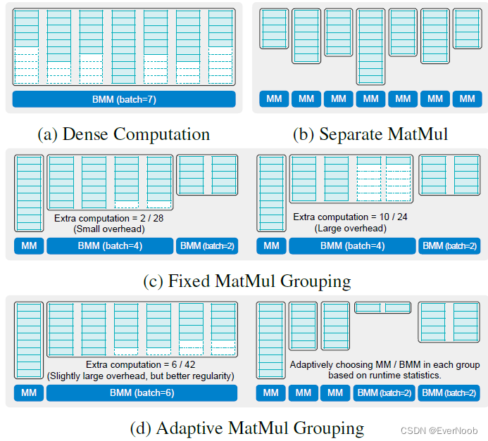
Figure 6: Illustration for different MatMul grouping strategies in TorchSparse (c, d) comparing with baselines (a: large FLOPs overhead, b: low device utilization, many kernel calls). Fixed grouping (c) trades FLOPs for regularity and adaptive grouping (d) searches for the best balance point.

Symmetric MatMul Grouping

With sparse workload, the map sizes for different weights within one SparseConv layer are usually different, as opposed to the dense workload (Figure 6a). However, for submanifold (stride=1) layers with odd kernel sizes, it turns out that the maps corresponding to weight offset (a; b; c) will always have the same size as the maps corresponding to the symmetric weight offset (-a;-b;-c). For a map 

Therefore, we are able to group matmul workload for symmetric weight offsets together and naturally have a batch size of 2. Note that the matmul workload corresponding to weight offset (0; 0; 0) is processed separately since it does not require any explicit data movement. As indicated in Figure 7, the batch=2 matmul (13 groups) can already be up to 1.2x faster than separate matmul.

Figure 7: Trading FLOPs for computation regularity via batched matrix multiplication can potentially bring about 1.5x speedup in matmul.

==> recall, "batch" first appeared in the paper as:

"We first propose adaptive MM grouping to smartly batch the computation workloads from different kernel offsets together, trading #FLOPs for better regularity."

==> the 1 group configuration is dense conv. and obviously worse than the baseline SSC, which is the 26 group configuration.

Fixed MatMul Grouping

Though symmetric grouping works well in stride=1 SparseConv layers, it falls short in generalizing to layers with downsampling layers. Also, it cannot push the batch size to > 2, which means that we still have a large gap towards best GPU utilization in Figure 7. Nevertheless, we find that clear pattern exists in the map size statistics (Figure 12):

1. for submanifold layers, the maps corresponding to W0 to W3 tend to have similar sizes and the rest of the weights other than the middle one have similar sizes ==> the notation here is rather confusing, or rather the reference to fig.12 does not support this conclusion, just take the authors' words on this for now; 

2. for downsampling layers, the maps for all offsets have similar sizes.

Consequently, we can batch the computation into three groups accordingly (symmetric grouping is also enabled whenever possible). Within each group, we pad all features to the maximum size (Figure 6c). Fixed grouping generally works well when all features within the same group have similar sizes (Figure 6c left), and this usually happens in downsampling layers. But for submanifold layers (Figure 6c right), the padding overhead can sometimes be large despite the better regularity, resulting in wasted computation.

Adaptive MatMul Grouping

The major drawback of fixed grouping is that it does not adapt to individual samples. This is problematic since workload size distributions can vary greatly across different datasets (Figure 12). It is also very labor-intensive to design different grouping strategies for different layers, different networks on a diverse set of datasets and hardware. To this end, we also design an adaptive grouping algorithm (Figure 6d) that automatically determines the input-adaptive grouping strategy for a given layer on arbitrary workload.

 

recall:

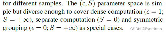
expressive power of the grouping's output space:

for the optimal set of adaptation hyper-parameter:

For a given SparseConvNet, we determine (epsilon; S) for each layer on a target dataset and hardware platform via exhaustive grid search on a small subset (usually 100 samples) of the training set.

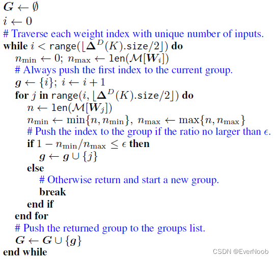
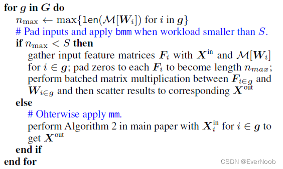
Group Matrix Multiplication, the Algorithm

==> group/grouped not batch/batched, bmm is performed with group; the naming inevitably gets awkward, bear the terms in mind.

We describe the process of applying the adaptive grouping strategies for each layer in Algorithm 4, which is performed via two steps.

First, we maintain two pointers to track the start and the end of the current group. Once redundancy ratio updated by the end pointer exceeds the tolerance of redundant computation epsilon, we return the working group to the groups list and move pointers to start a new group.

Second, for each group, we determine if batched matmul is performed on it based on the value of S.

 

 

Adaptive Strategy Search

i.e. the search for the proper value of the hyper-parameter set (epsilon, S)

 

 ==> the search space is inference only !! so that no optimization is needed when deployed; and inference time is about the only timing we care about.

Data Movement Optimization

Quantized and Vectorized Memory Access

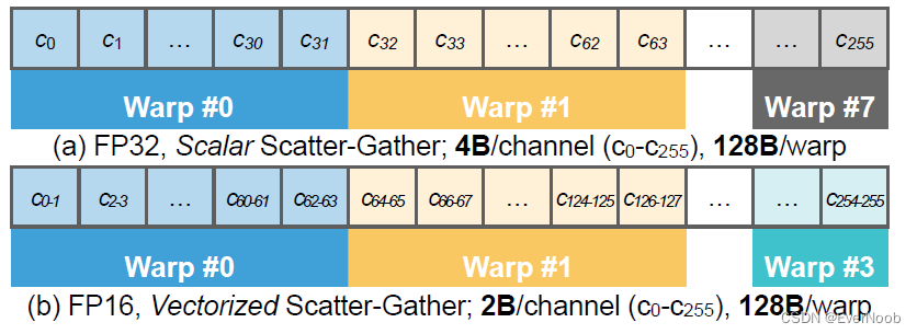
Figure 8: TorchSparse applies vectorized and quantized scatter-gather to greatly data movement latency.

==> the gist is that quantization from f32 to f16 cannot by itself reduce mem. access due to NVIDIA's hardware access rules; vectorize the datum is necessary for a ~2x gain.

==> furthermore, the NVIDIA's scatter mechanics renders the quantization to INT8 pointless.

Fused and Locality-Aware Memory Access

key idea: reduce cache misses and hence the repetitive costly gather/scatter operations 

1. fuse up gather/scatter

2. reorder accesses

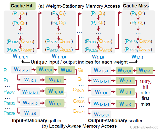
Figure 9: TorchSparse proposes cache-friendly locality-aware memory access pattern. In contrary, baseline implementation (a) cannot exploit cache reuse due to uniqueness in input/output indices for each weight.

Estimation and Notation

Operation Fusion

As is shown in Algorithm 2 and Figure 9a, the current implementation completely separates gather/scatter for different weights. When we perform gather operation for W_k+1, the GPU cache is filled with scatter buffer features forWk as long as the GPU cache size is much smaller than N1 (the typically > 40MB, much larger than the 5.5MB L2 cache of NVIDIA RTX 2080 Ti). Intuitively, for gather operation on W_k+1, we hope that the cache is filled with gather buffer features from W_k. ==>

first fuse all gather operations before matrix multiplication,

and fuse all scatter operations afterwards.

==> we don't care about latency for a single partial sum, only the overall inference time

As such, the GPU cache will always hold data from the same type of buffer.

Memory Access Order

In the weight-stationary / map order (Figure 9a), all map entries for weight W_k are unique, so there is no chance of feature reuse and each gather/scatter will be a cache miss. As is shown in Figure 9b, we instead take a locality-aware memory access order. We gather the input features in the input-stationary order and scatter the partial sums in the output stationary order.

 ==> W_k in order to P_i BFS traversal

Mapping Optimization

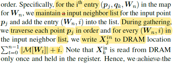
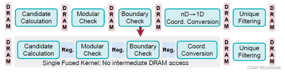
We first choose the map search strategy for each layer from [grid, hashmap] in a similar manner to adaptive grouping. Here, grid corresponds to a naive collision-free hashmap described in Section 2.1.2; it takes larger memory space but hashmap construction / query requires exactly 1 DRAM access per-entry, smaller than conventional hashmaps. We then perform kernel fusion (Figure 10) on output coordinates computation for downsampling. The downsample operation applies a sliding window around each point and

1. calculate candidate activated points with broadcast add;

2. perform modular check;

3. perform boundary check and generate a mask on whether each point is kept;

4. converts the remaining candidate point coordinates to 1D values;

5. perform unique operation to keep final output coordinates (detailed in Appendix A).

There are DRAM accesses between every two of the five stages, making downsampling kernels memory-bounded. We therefore fuse stages 1 to 4 in a single kernel and use registers to store intermediate results, which eliminates all intermediate DRAM write. For the fused kernel, we further perform control logic simplification, full loop unrolling and utilize the symmetry of submanifold maps. Overall, the mapping operations are accelerated by 4.6x on detection tasks after our optimization.

Figure 10: TorchSparse reduces mapping DRAM access and improves mapping latency via kernel fusion.

==> clearly it doesn't make much sense to set the DRAM access granularity to per point; this issue likely arose due to traditional CPU/GPU architecture does not explicitly expose register control to the programmer.