【相机畸变：Brown-Conrady、Kanala-Brandt畸变模型与迭代去畸变】

置顶 memmolo

已于 2024-01-05 11:19:50 修改

阅读量2.6k

点赞数 8

文章标签：计算机视觉图像处理

于 2023-07-13 10:24:40 首次发布

本文链接：https://blog.csdn.net/memmolo/article/details/131676699

版权

介绍

本文介绍计算机视觉中常用的两种相机畸变模型：Brown-Conrady畸变模型和Kanala-Brandt畸变模型，以及点去畸变的迭代方法及其Matlab实现。

Brown/Brown-Conrady畸变模型

畸变模型

Brown-Conrady模型中，无畸变点坐标 $(x, y)$ 到畸变点坐标 $x_d,y_d)$ 的变换关系表示为： $r^2=x^2+y^2\\x_d=x(\frac{1+k_1r^2+k_2r^4+k_3r^6}{1+k_4r^2+k_5r^4+k_6r^6})+2p_1xy+p_2(r^2+2x^2)\\y_d=y(\frac{1+k_1r^2+k_2r^4+k_3r^6}{1+k_4r^2+k_5r^4+k_6r^6})+p_1(r^2+2y^2)+2p_2xy$ 其中， $x(\frac{1+k_1r^2+k_2r^4+k_3r^6}{1+k_4r^2+k_5r^4+k_6r^6})$ 和 $y(\frac{1+k_1r^2+k_2r^4+k_3r^6}{1+k_4r^2+k_5r^4+k_6r^6})$ 为径向畸变项， $k_1,k_2,k_3,k_4,k_5,k_6$ 为径向畸变系数； $2p_1xy+p_2(r^2+2x^2)$ 和 $p_1(r^2+2y^2)+2p_2xy$ 为切向畸变项， $p_1,p_2$ 为切向畸变系数（注：这个畸变项通常称为切向畸变，但实际畸变方向并非沿切向，也有径向成分。这个畸变项实际是失心畸变，表示镜头光轴与图像靶面不垂直引入的畸变，至于为什么是这个形式可以参阅文献【3】（很难看懂-.-），失心畸变后来由Brown引入计算机视觉领域，参阅文献【4-5】）。
常规镜头畸变较小，Brown-Conrady模型的径向畸变系数通常使用至 $k_2$ 或 $k_3$ ；对于大视场角镜头或鱼眼镜头，径向畸变系数需使用至 $k_6$ 以保证边缘拟合效果。

点去畸变

现已知 $x_d,y_d)$ 和畸变参数，想要得到 $(x, y)$ ，需要通过迭代求解，迭代过程如下
初值： $x_0=x_d\\y_0=y_d$ 迭代公式（固定点迭代）： $x_{n+1}=[x_d-2p_1x_ny_n-p_2(r_n^2+2x_n^2)]\cdot\frac{1+k_4r_n^2+k_5r_n^4+k_6r_n^6}{1+k_1r_n^2+k_2r_n^4+k_3r_n^6}\\y_{n+1}=[y_d-p_1(r_n^2+2y_n^2)-2p_2x_ny_n]\cdot\frac{1+k_4r_n^2+k_5r_n^4+k_6r_n^6}{1+k_1r_n^2+k_2r_n^4+k_3r_n^6}$

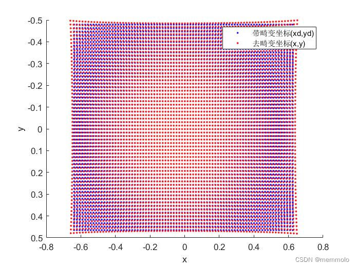
Matlab实现

clear
clc
% 设定图像大小
w = 640;
h = 480;
% 设定焦距
fx = 500;
fy = 500;
% 设定主点
cx = (w-1)/2;
cy = (h-1)/2;
% 随机生成畸变
rng(100); %随机数种子
k1 = 0.1*randn(1);
k2 = 0.1*randn(1);
k3 = 0.1*randn(1);
k4 = 0.1*randn(1);
k5 = 0.1*randn(1);
k6 = 0.1*randn(1);
p1 = 0.001*randn(1);
p2 = 0.001*randn(1);
% 迭代次数
iter_num = 30;
% 采样步长，为了减少绘图点的密度
sampling_step = 8;
% 生成xd、yd
[ud, vd] = meshgrid(0:sampling_step:w-1,0:sampling_step:h-1);
xd = (ud-cx)/fx;
yd = (vd-cy)/fy;
% 去畸变迭代
x = xd;
y = yd;
for i = 1:iter_num
    r2 = x.^2+y.^2;
    x = (xd-(p1*(2*x.*y)+p2*(r2+2*x.^2)))./(1+k1*r2+k2*r2.^2+k3*r2.^3).*(1+k4*r2+k5*r2.^2+k6*r2.^3);
    y = (yd-(p1*(r2+2*y.^2)+p2*(2*x.*y)))./(1+k1*r2+k2*r2.^2+k3*r2.^3).*(1+k4*r2+k5*r2.^2+k6*r2.^3);
end
% 绘图
figure, hold on
scatter(xd(:),yd(:),'b.')
scatter(x(:),y(:),'r.')
legend('带畸变坐标(xd,yd)','去畸变坐标(x,y)')
axis ij
xlabel('x')
ylabel('y')

Brown-Conrady模型去畸变

KB/Kanala-Brandt畸变模型

畸变模型

对于理想的透视投影，或者一个无畸变的镜头，光线入射角 $\theta$ 与其最终投影在相机靶面位置 $D$ 的关系可以表示为 $D=f\tan(\theta)$ 其中， $f$ 为镜头的物理焦距。可以看出，相机靶面大小固定时，焦距越小，可以拍摄的视场越大，因此大视场角镜头通常为短焦镜头。当焦距也固定时，想要拍摄大的视场，则需要通过改变镜头设计，改变 $\theta$ 与 $D$ 的映射关系，来增大视场。
鱼眼镜头为了拍摄更大视场角，常遵循以下几种设计准则

等距投影（equidistance projection）： $D=f\theta$
立体投影（stereographic projection）： $D=2f\tan(\theta/2)$
等立体角投影（equisolid angle projection）： $D=2f\sin(\theta/2)$
正交投影（orthogonal projection）： $D=f\sin(\theta)$

用 $r$ 表示理想透视投影中归一化平面坐标，则有 $r=D/f=\tan(\theta)$ 以等距投影为例，畸变坐标 $r_d$ 与 $r$ 的关系表示为 $r_d=\theta=\arctan(r)$ 若继续按照Brown畸变模型中的多项式 $r_d=r+k_1r^3+k_2r^5+...$ 进行拟合，由于 $\arctan(r)$ 的展开特性，只使用少量系数拟合的话，图像边缘的拟合效果是非常差的。所以Brown-Conrady模型采用了如下拟合方式 $r_d= r\frac{1+ k_1r^2+k_2r^4+k_3r^6}{1+ k_4r^2+k_5r^4+k_6r^6}$ 进行改进。而Kanala-Brandt模型则不同，研究者注意到鱼眼镜头的设计特点，使用 $\theta$ 的多项式而非 $r$ 的多项式进行拟合 $r_d = \theta+k_1\theta^3+k_2\theta^5+...$ 因此Kanala-Brandt模型中，无畸变点坐标 $(x, y)$ 到畸变点坐标 $x_d,y_d)$ 的变换关系表示为： $r^2=x^2+y^2\\\theta = atan(r)\\r_d=\theta(1+k_1\theta^2+k_2\theta^4+k_3\theta^6+k_4\theta^8)\\x_d=r_d\cdot x/r\\y_d=r_d\cdot y/r$

点去畸变

初值： $\theta_0=r_d$ 迭代公式（牛顿法）： $\theta_{n+1}=\theta_n-\Delta\theta_n\\\Delta\theta_n=\frac{\theta_n+k_1\theta_n^3+k_2\theta_n^5+k_3\theta_n^7+k_4\theta_n^9-r_d}{1+3k_1\theta_n^2+5k_2\theta_n^4+7k_3\theta_n^6+9k_4\theta_n^8}$ 去畸变坐标为： $x=\frac{x_d}{r_d}\tan(\theta)\\y=\frac{y_d}{r_d}\tan(\theta)$

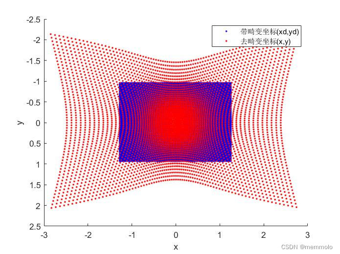
Matlab实现

clear
clc
% 设定图像大小
w = 640;
h = 480;
% 设定焦距
fx = 250;
fy = 250;
% 设定主点
cx = (w-1)/2;
cy = (h-1)/2;
% 随机生成畸变
rng(100); %随机数种子
k1 = 0.1*randn(1);
k2 = 0.1*randn(1);
k3 = 0.1*randn(1);
k4 = 0.1*randn(1);
% 迭代次数
iter_num = 30;
% 采样步长，为了减少绘图点的密度
sampling_step = 8;
% 生成xd、yd
[ud, vd] = meshgrid(0:sampling_step:w-1,0:sampling_step:h-1);
xd = (ud-cx)/fx;
yd = (vd-cy)/fy;
% 去畸变迭代
rd = sqrt(xd.^2+yd.^2);
theta = rd;
for i=1:iter_num
    theta_fix = (theta+k1*theta.^3+k2*theta.^5+k3*theta.^7+k4*theta.^9-rd)./...
        (1+3*k1*theta.^2+5*k2*theta.^4+7*k3*theta.^6+9*k4*theta.^8);
    theta = theta-theta_fix;
end
scale = tan(theta)./rd;
x = xd.*scale;
y = yd.*scale;
% 绘图
figure, hold on
scatter(xd(:),yd(:),'b.')
scatter(x(:),y(:),'r.')
legend('带畸变坐标(xd,yd)','去畸变坐标(x,y)')
axis ij
xlabel('x')
ylabel('y')

Kanala-Brandt模型去畸变

OpenCV去畸变程序

这里补充OpenCV4.9去畸变程序作为参考。

Brown/Brown-Conrady畸变模型

static void cvUndistortPointsInternal( const CvMat* _src, CvMat* _dst, const CvMat* _cameraMatrix,
                   const CvMat* _distCoeffs,
                   const CvMat* matR, const CvMat* matP, cv::TermCriteria criteria)
{
    CV_Assert(criteria.isValid());
    double A[3][3], RR[3][3], k[14]={0,0,0,0,0,0,0,0,0,0,0,0,0,0};
    CvMat matA=cvMat(3, 3, CV_64F, A), _Dk;
    CvMat _RR=cvMat(3, 3, CV_64F, RR);
    cv::Matx33d invMatTilt = cv::Matx33d::eye();
    cv::Matx33d matTilt = cv::Matx33d::eye();

    CV_Assert( CV_IS_MAT(_src) && CV_IS_MAT(_dst) &&
        (_src->rows == 1 || _src->cols == 1) &&
        (_dst->rows == 1 || _dst->cols == 1) &&
        _src->cols + _src->rows - 1 == _dst->rows + _dst->cols - 1 &&
        (CV_MAT_TYPE(_src->type) == CV_32FC2 || CV_MAT_TYPE(_src->type) == CV_64FC2) &&
        (CV_MAT_TYPE(_dst->type) == CV_32FC2 || CV_MAT_TYPE(_dst->type) == CV_64FC2));

    CV_Assert( CV_IS_MAT(_cameraMatrix) &&
        _cameraMatrix->rows == 3 && _cameraMatrix->cols == 3 );

    cvConvert( _cameraMatrix, &matA );


    if( _distCoeffs )
    {
        CV_Assert( CV_IS_MAT(_distCoeffs) &&
            (_distCoeffs->rows == 1 || _distCoeffs->cols == 1) &&
            (_distCoeffs->rows*_distCoeffs->cols == 4 ||
             _distCoeffs->rows*_distCoeffs->cols == 5 ||
             _distCoeffs->rows*_distCoeffs->cols == 8 ||
             _distCoeffs->rows*_distCoeffs->cols == 12 ||
             _distCoeffs->rows*_distCoeffs->cols == 14));

        _Dk = cvMat( _distCoeffs->rows, _distCoeffs->cols,
            CV_MAKETYPE(CV_64F,CV_MAT_CN(_distCoeffs->type)), k);

        cvConvert( _distCoeffs, &_Dk );
        if (k[12] != 0 || k[13] != 0)
        {
            cv::detail::computeTiltProjectionMatrix<double>(k[12], k[13], NULL, NULL, NULL, &invMatTilt);
            cv::detail::computeTiltProjectionMatrix<double>(k[12], k[13], &matTilt, NULL, NULL);
        }
    }

    if( matR )
    {
        CV_Assert( CV_IS_MAT(matR) && matR->rows == 3 && matR->cols == 3 );
        cvConvert( matR, &_RR );
    }
    else
        cvSetIdentity(&_RR);

    if( matP )
    {
        double PP[3][3];
        CvMat _P3x3, _PP=cvMat(3, 3, CV_64F, PP);
        CV_Assert( CV_IS_MAT(matP) && matP->rows == 3 && (matP->cols == 3 || matP->cols == 4));
        cvConvert( cvGetCols(matP, &_P3x3, 0, 3), &_PP );
        cvMatMul( &_PP, &_RR, &_RR );
    }

    const CvPoint2D32f* srcf = (const CvPoint2D32f*)_src->data.ptr;
    const CvPoint2D64f* srcd = (const CvPoint2D64f*)_src->data.ptr;
    CvPoint2D32f* dstf = (CvPoint2D32f*)_dst->data.ptr;
    CvPoint2D64f* dstd = (CvPoint2D64f*)_dst->data.ptr;
    int stype = CV_MAT_TYPE(_src->type);
    int dtype = CV_MAT_TYPE(_dst->type);
    int sstep = _src->rows == 1 ? 1 : _src->step/CV_ELEM_SIZE(stype);
    int dstep = _dst->rows == 1 ? 1 : _dst->step/CV_ELEM_SIZE(dtype);

    double fx = A[0][0];
    double fy = A[1][1];
    double ifx = 1./fx;
    double ify = 1./fy;
    double cx = A[0][2];
    double cy = A[1][2];

    int n = _src->rows + _src->cols - 1;
    for( int i = 0; i < n; i++ )
    {
        double x, y, x0 = 0, y0 = 0, u, v;
        if( stype == CV_32FC2 )
        {
            x = srcf[i*sstep].x;
            y = srcf[i*sstep].y;
        }
        else
        {
            x = srcd[i*sstep].x;
            y = srcd[i*sstep].y;
        }
        u = x; v = y;
        x = (x - cx)*ifx;
        y = (y - cy)*ify;

        if( _distCoeffs ) {
            // compensate tilt distortion
            cv::Vec3d vecUntilt = invMatTilt * cv::Vec3d(x, y, 1);
            double invProj = vecUntilt(2) ? 1./vecUntilt(2) : 1;
            x0 = x = invProj * vecUntilt(0);
            y0 = y = invProj * vecUntilt(1);

            double error = std::numeric_limits<double>::max();
            // compensate distortion iteratively
            // 去畸变核心代码
            for( int j = 0; ; j++ )
            {
                if ((criteria.type & cv::TermCriteria::COUNT) && j >= criteria.maxCount)
                    break;
                if ((criteria.type & cv::TermCriteria::EPS) && error < criteria.epsilon)
                    break;
                double r2 = x*x + y*y;
                double icdist = (1 + ((k[7]*r2 + k[6])*r2 + k[5])*r2)/(1 + ((k[4]*r2 + k[1])*r2 + k[0])*r2);
                if (icdist < 0)  // test: undistortPoints.regression_14583
                {
                    x = (u - cx)*ifx;
                    y = (v - cy)*ify;
                    break;
                }
                double deltaX = 2*k[2]*x*y + k[3]*(r2 + 2*x*x)+ k[8]*r2+k[9]*r2*r2;
                double deltaY = k[2]*(r2 + 2*y*y) + 2*k[3]*x*y+ k[10]*r2+k[11]*r2*r2;
                x = (x0 - deltaX)*icdist;
                y = (y0 - deltaY)*icdist;

                if(criteria.type & cv::TermCriteria::EPS)
                {
                    double r4, r6, a1, a2, a3, cdist, icdist2;
                    double xd, yd, xd0, yd0;
                    cv::Vec3d vecTilt;

                    r2 = x*x + y*y;
                    r4 = r2*r2;
                    r6 = r4*r2;
                    a1 = 2*x*y;
                    a2 = r2 + 2*x*x;
                    a3 = r2 + 2*y*y;
                    cdist = 1 + k[0]*r2 + k[1]*r4 + k[4]*r6;
                    icdist2 = 1./(1 + k[5]*r2 + k[6]*r4 + k[7]*r6);
                    xd0 = x*cdist*icdist2 + k[2]*a1 + k[3]*a2 + k[8]*r2+k[9]*r4;
                    yd0 = y*cdist*icdist2 + k[2]*a3 + k[3]*a1 + k[10]*r2+k[11]*r4;

                    vecTilt = matTilt*cv::Vec3d(xd0, yd0, 1);
                    invProj = vecTilt(2) ? 1./vecTilt(2) : 1;
                    xd = invProj * vecTilt(0);
                    yd = invProj * vecTilt(1);

                    double x_proj = xd*fx + cx;
                    double y_proj = yd*fy + cy;

                    error = sqrt( pow(x_proj - u, 2) + pow(y_proj - v, 2) );
                }
            }
        }

        double xx = RR[0][0]*x + RR[0][1]*y + RR[0][2];
        double yy = RR[1][0]*x + RR[1][1]*y + RR[1][2];
        double ww = 1./(RR[2][0]*x + RR[2][1]*y + RR[2][2]);
        x = xx*ww;
        y = yy*ww;

        if( dtype == CV_32FC2 )
        {
            dstf[i*dstep].x = (float)x;
            dstf[i*dstep].y = (float)y;
        }
        else
        {
            dstd[i*dstep].x = x;
            dstd[i*dstep].y = y;
        }
    }
}

KB/Kanala-Brandt畸变模型

void cv::fisheye::undistortPoints( InputArray distorted, OutputArray undistorted, InputArray K, InputArray D,
                                   InputArray R, InputArray P, TermCriteria criteria)
{
    CV_INSTRUMENT_REGION();

    // will support only 2-channel data now for points
    CV_Assert(distorted.type() == CV_32FC2 || distorted.type() == CV_64FC2);
    undistorted.create(distorted.size(), distorted.type());

    CV_Assert(P.empty() || P.size() == Size(3, 3) || P.size() == Size(4, 3));
    CV_Assert(R.empty() || R.size() == Size(3, 3) || R.total() * R.channels() == 3);
    CV_Assert(D.total() == 4 && K.size() == Size(3, 3) && (K.depth() == CV_32F || K.depth() == CV_64F));

    CV_Assert(criteria.isValid());

    cv::Vec2d f, c;
    if (K.depth() == CV_32F)
    {
        Matx33f camMat = K.getMat();
        f = Vec2f(camMat(0, 0), camMat(1, 1));
        c = Vec2f(camMat(0, 2), camMat(1, 2));
    }
    else
    {
        Matx33d camMat = K.getMat();
        f = Vec2d(camMat(0, 0), camMat(1, 1));
        c = Vec2d(camMat(0, 2), camMat(1, 2));
    }

    Vec4d k = D.depth() == CV_32F ? (Vec4d)*D.getMat().ptr<Vec4f>(): *D.getMat().ptr<Vec4d>();

    cv::Matx33d RR = cv::Matx33d::eye();
    if (!R.empty() && R.total() * R.channels() == 3)
    {
        cv::Vec3d rvec;
        R.getMat().convertTo(rvec, CV_64F);
        RR = cv::Affine3d(rvec).rotation();
    }
    else if (!R.empty() && R.size() == Size(3, 3))
        R.getMat().convertTo(RR, CV_64F);

    if(!P.empty())
    {
        cv::Matx33d PP;
        P.getMat().colRange(0, 3).convertTo(PP, CV_64F);
        RR = PP * RR;
    }

    // start undistorting
    const cv::Vec2f* srcf = distorted.getMat().ptr<cv::Vec2f>();
    const cv::Vec2d* srcd = distorted.getMat().ptr<cv::Vec2d>();
    cv::Vec2f* dstf = undistorted.getMat().ptr<cv::Vec2f>();
    cv::Vec2d* dstd = undistorted.getMat().ptr<cv::Vec2d>();

    size_t n = distorted.total();
    int sdepth = distorted.depth();

    const bool isEps = (criteria.type & TermCriteria::EPS) != 0;

    /* Define max count for solver iterations */
    int maxCount = std::numeric_limits<int>::max();
    if (criteria.type & TermCriteria::MAX_ITER) {
        maxCount = criteria.maxCount;
    }


    for(size_t i = 0; i < n; i++ )
    {
        Vec2d pi = sdepth == CV_32F ? (Vec2d)srcf[i] : srcd[i];  // image point
        Vec2d pw((pi[0] - c[0])/f[0], (pi[1] - c[1])/f[1]);      // world point

        double theta_d = sqrt(pw[0]*pw[0] + pw[1]*pw[1]);

        // the current camera model is only valid up to 180 FOV
        // for larger FOV the loop below does not converge
        // clip values so we still get plausible results for super fisheye images > 180 grad
        theta_d = min(max(-CV_PI/2., theta_d), CV_PI/2.);

        bool converged = false;
        double theta = theta_d;

        double scale = 0.0;

        if (!isEps || fabs(theta_d) > criteria.epsilon)
        {
            // compensate distortion iteratively using Newton method
            // 去畸变核心代码
            for (int j = 0; j < maxCount; j++)
            {
                double theta2 = theta*theta, theta4 = theta2*theta2, theta6 = theta4*theta2, theta8 = theta6*theta2;
                double k0_theta2 = k[0] * theta2, k1_theta4 = k[1] * theta4, k2_theta6 = k[2] * theta6, k3_theta8 = k[3] * theta8;
                /* new_theta = theta - theta_fix, theta_fix = f0(theta) / f0'(theta) */
                double theta_fix = (theta * (1 + k0_theta2 + k1_theta4 + k2_theta6 + k3_theta8) - theta_d) /
                                   (1 + 3*k0_theta2 + 5*k1_theta4 + 7*k2_theta6 + 9*k3_theta8);
                theta = theta - theta_fix;

                if (isEps && (fabs(theta_fix) < criteria.epsilon))
                {
                    converged = true;
                    break;
                }
            }

            scale = std::tan(theta) / theta_d;
        }
        else
        {
            converged = true;
        }

        // theta is monotonously increasing or decreasing depending on the sign of theta
        // if theta has flipped, it might converge due to symmetry but on the opposite of the camera center
        // so we can check whether theta has changed the sign during the optimization
        bool theta_flipped = ((theta_d < 0 && theta > 0) || (theta_d > 0 && theta < 0));

        if ((converged || !isEps) && !theta_flipped)
        {
            Vec2d pu = pw * scale; //undistorted point

            // reproject
            Vec3d pr = RR * Vec3d(pu[0], pu[1], 1.0); // rotated point optionally multiplied by new camera matrix
            Vec2d fi(pr[0]/pr[2], pr[1]/pr[2]);       // final

            if( sdepth == CV_32F )
                dstf[i] = fi;
            else
                dstd[i] = fi;
        }
        else
        {
            // Vec2d fi(std::numeric_limits<double>::quiet_NaN(), std::numeric_limits<double>::quiet_NaN());
            Vec2d fi(-1000000.0, -1000000.0);

            if( sdepth == CV_32F )
                dstf[i] = fi;
            else
                dstd[i] = fi;
        }
    }
}

参考资料

Brown-Conrady畸变模型
【1】OpenCV相机模型介绍：https://docs.opencv.org/3.4/d9/d0c/group__calib3d.html
【2】OpenCV去畸变函数：cvUndistortPointsInternal
【3】Conrady A E. Lens-systems, decentered[J]. Monthly Notices of the Royal Astronomical Society, Vol. 79, p. 384-390, 1919, 79: 384-390.
【4】Brown D C. Decentering distortion of lenses, D. Brown Associates[J]. Inc, Eau Gallie, Florida, Tech. Rep, 1966.
【5】Duane C B. Close-range camera calibration[J]. Photogramm. Eng, 1971, 37(8): 855-866.
【6】Weng J, Cohen P, Herniou M. Camera calibration with distortion models and accuracy evaluation[J]. IEEE Transactions on pattern analysis and machine intelligence, 1992, 14(10): 965-980.
Kanala-Brandt畸变模型
【7】OpenCV相机模型介绍：https://docs.opencv.org/3.4/db/d58/group__calib3d__fisheye.html
【8】OpenCV去畸变函数：cv::fisheye::undistortPoints
【9】Kannala J, Brandt S. A generic camera calibration method for fish-eye lenses[C]//Proceedings of the 17th International Conference on Pattern Recognition, 2004. ICPR 2004. IEEE, 2004, 1: 10-13.
【10】Kannala J, Brandt S S. A generic camera model and calibration method for conventional, wide-angle, and fish-eye lenses[J]. IEEE transactions on pattern analysis and machine intelligence, 2006, 28(8): 1335-1340.

memmolo

关注

8
点赞
踩
26

收藏

觉得还不错? 一键收藏
4
评论
【相机畸变：Brown-Conrady、Kanala-Brandt畸变模型与迭代去畸变】

本文介绍计算机视觉中常用的两种相机畸变模型：Brown-Conrady畸变模型和Kanala-Brandt畸变模型，以及点去畸变的迭代方法及其Matlab实现。
复制链接

扫一扫