时间序列预测实操（从0到1）

watersink

已于 2025-03-06 17:16:50 修改

阅读量141

点赞数 2

分类专栏：深度学习机器学习文章标签： python 开发语言

于 2025-03-06 17:10:48 首次发布

本文链接：https://blog.csdn.net/qq_14845119/article/details/146075080

版权

深度学习同时被 2 个专栏收录

55 篇文章

订阅专栏

机器学习

17 篇文章

订阅专栏

import pandas as pd
df = pd.read_csv('stock.csv')
print(df)

           date   open   high    low  close     volume
0      2020/1/3  55.15  55.38  54.25  54.25   91498808
1      2020/1/4  56.43  56.53  55.05  55.05   75189048
2      2020/1/5  56.32  56.40  55.35  55.45   39782132
3      2020/1/6  55.69  56.93  55.03  56.36   66463320
4      2020/1/7  56.15  56.45  55.90  56.40   35874840
..          ...    ...    ...    ...    ...        ...
691  2021/11/24  25.01  26.33  24.86  26.28  178976576
692  2021/11/25  24.98  25.22  24.71  25.11   53494888
693  2021/11/26  24.08  25.03  24.08  24.91   62335408
694  2021/11/27  23.63  24.42  23.29  23.99   40682752
695  2021/11/28  23.78  23.88  22.54  23.74   66763176

[696 rows x 6 columns]

df.dropna(inplace=True)
print(df)

           date   open   high    low  close     volume
0      2020/1/3  55.15  55.38  54.25  54.25   91498808
1      2020/1/4  56.43  56.53  55.05  55.05   75189048
2      2020/1/5  56.32  56.40  55.35  55.45   39782132
3      2020/1/6  55.69  56.93  55.03  56.36   66463320
4      2020/1/7  56.15  56.45  55.90  56.40   35874840
..          ...    ...    ...    ...    ...        ...
691  2021/11/24  25.01  26.33  24.86  26.28  178976576
692  2021/11/25  24.98  25.22  24.71  25.11   53494888
693  2021/11/26  24.08  25.03  24.08  24.91   62335408
694  2021/11/27  23.63  24.42  23.29  23.99   40682752
695  2021/11/28  23.78  23.88  22.54  23.74   66763176

[695 rows x 6 columns]

# 拆分训练集和验证集(数据较大，进行归一化处理)
X = df.loc[df['close'].notnull(),df.columns[1:]]
Y = df.loc[df['close'].notnull(),df.columns[-2]]
print(X)
print(Y)

      open   high    low  close     volume
0    55.15  55.38  54.25  54.25   91498808
1    56.43  56.53  55.05  55.05   75189048
2    56.32  56.40  55.35  55.45   39782132
3    55.69  56.93  55.03  56.36   66463320
4    56.15  56.45  55.90  56.40   35874840
..     ...    ...    ...    ...        ...
691  25.01  26.33  24.86  26.28  178976576
692  24.98  25.22  24.71  25.11   53494888
693  24.08  25.03  24.08  24.91   62335408
694  23.63  24.42  23.29  23.99   40682752
695  23.78  23.88  22.54  23.74   66763176

[695 rows x 5 columns]
0      54.25
1      55.05
2      55.45
3      56.36
4      56.40
       ...  
691    26.28
692    25.11
693    24.91
694    23.99
695    23.74
Name: close, Length: 695, dtype: float64

import numpy as np
sequence_length = 9
X = X.to_numpy().astype(np.float32)
Y = Y.to_numpy().astype(np.float32)

X_lists = []
for i in range(X.shape[0]-sequence_length):
    X_lists.append(X[i:i+sequence_length,:])

X=np.array(X_lists)


Y = Y[sequence_length:]
print(X.shape)
print(Y.shape)

(686, 9, 5)
(686,)

import numpy as np
mean_X = np.mean(X, axis = 0)
std_X = np.std(X, axis=0)
normalized_X = (X-mean_X)/std_X

mean_Y = np.mean(Y)
std_Y = np.std(Y)
normalized_Y = (Y-mean_Y)/std_Y
#normalized_Y = np.expand_dims(normalized_Y, 1)

print(normalized_X.shape, normalized_Y.shape)

(686, 9, 5) (686,)
<ipython-input-8-77884a25ccaf>:4: RuntimeWarning: invalid value encountered in true_divide
  normalized_X = (X-mean_X)/std_X

from sklearn.model_selection import train_test_split
test_size = 0.1
train_x,test_x,train_y,test_y = train_test_split(normalized_X,normalized_Y,test_size=test_size,shuffle=False)
print(train_x.shape,test_x.shape,train_y.shape,test_y.shape)

(617, 9, 5) (69, 9, 5) (617,) (69,)

import torch
import torch.nn as nn

# 创建LSTM模型
class Lstm(nn.Module):
    
    def __init__(self,feature_size,hidden_size,num_layers):
        super(Lstm,self).__init__()
        self.lstm = nn.LSTM(input_size=feature_size,hidden_size=hidden_size,num_layers=num_layers,batch_first=True)
        
        self.linear = nn.Linear(in_features=hidden_size*sequence_length,out_features=1)
    
    def forward(self,x):
        out,(hn,cn)= self.lstm(x)
        out = out.reshape(-1,hidden_size*sequence_length )
        z = self.linear(out)
        z = torch.squeeze(z)
        return z 



from torch.nn import MSELoss
from torch.optim import Adam,SGD,RMSprop
# 实例化模型    
feature_size = 5 
hidden_size = 32
num_layers = 2 
lstm = Lstm(feature_size=feature_size,hidden_size=hidden_size,num_layers=num_layers)

 
# 设置损失函数和优化函数
Loss = MSELoss()

opt = Adam(params=lstm.parameters(),lr=0.001)



# 开始训练
epochs = 300 
loss_lists = []

train_x_tensor = torch.from_numpy(train_x)
train_y_tensor = torch.from_numpy(train_y)
test_x_tensor = torch.from_numpy(test_x)
test_y_tensor = torch.from_numpy(test_y)

for epoch in range(epochs):
    out = lstm(train_x_tensor) 
    loss_value = Loss(out,train_y_tensor)
    opt.zero_grad()
    loss_value.backward()
    opt.step()
    
    print("epoch:{} loss:{}".format(epoch,loss_value))
    loss_lists.append(loss_value)

epoch:0 loss:0.9820637702941895
epoch:1 loss:0.9601344466209412
epoch:2 loss:0.9402551651000977
epoch:3 loss:0.9215231537818909
epoch:4 loss:0.9033159613609314
epoch:5 loss:0.8851599097251892
epoch:6 loss:0.8666412234306335
epoch:7 loss:0.8473861813545227
epoch:8 loss:0.8270445466041565
epoch:9 loss:0.8052817583084106
epoch:10 loss:0.781779408454895
epoch:11 loss:0.7562394142150879
epoch:12 loss:0.7283873558044434
epoch:13 loss:0.6979731321334839
epoch:14 loss:0.6647756099700928
epoch:15 loss:0.6286104917526245
epoch:16 loss:0.5893445014953613
epoch:17 loss:0.546915590763092
epoch:18 loss:0.5013647079467773
epoch:19 loss:0.45287951827049255
epoch:20 loss:0.4018512964248657
epoch:21 loss:0.3489430248737335
epoch:22 loss:0.29516512155532837
epoch:23 loss:0.2419436126947403
epoch:24 loss:0.19114260375499725
...
epoch:231 loss:0.015521089546382427
epoch:232 loss:0.015496882610023022
epoch:233 loss:0.015472659841179848
epoch:234 loss:0.01544840820133686
Output is truncated. View as a scrollable element or open in a text editor. Adjust cell output settings...
epoch:235 loss:0.015424135141074657
epoch:236 loss:0.015399832278490067
epoch:237 loss:0.015375500544905663
epoch:238 loss:0.01535114087164402
epoch:239 loss:0.015326756983995438
epoch:240 loss:0.015302336774766445
epoch:241 loss:0.015277883969247341
epoch:242 loss:0.0152533994987607
epoch:243 loss:0.015228882431983948
epoch:244 loss:0.015204326249659061
epoch:245 loss:0.015179736539721489
epoch:246 loss:0.015155103988945484
epoch:247 loss:0.015130436979234219
epoch:248 loss:0.015105726197361946
epoch:249 loss:0.01508097443729639
epoch:250 loss:0.015056180767714977
epoch:251 loss:0.015031341463327408
epoch:252 loss:0.015006458386778831
epoch:253 loss:0.014981526881456375
epoch:254 loss:0.01495654508471489
epoch:255 loss:0.014931514859199524
epoch:256 loss:0.014906435273587704
epoch:257 loss:0.014881305396556854
epoch:258 loss:0.014856117777526379
epoch:259 loss:0.01483087707310915
...
epoch:296 loss:0.013845087960362434
epoch:297 loss:0.013816643506288528
epoch:298 loss:0.013788075186312199
epoch:299 loss:0.013759390451014042
Output is truncated. View as a scrollable element or open in a text editor. Adjust cell output settings...

import matplotlib.pyplot as plt
plt.plot(loss_lists, label='loss')
plt.xlabel('iter')
plt.ylabel('loss')
plt.show()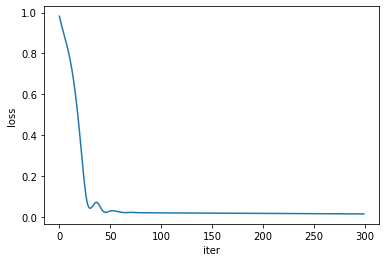

#模型eval
lstm.eval()
out_test = lstm(test_x_tensor) 
out_test = out_test.detach().numpy()
out_test = out_test*std_Y+mean_Y
label_test = test_y*std_Y+mean_Y
#画图
plt.plot(out_test, label='pred')
plt.plot(label_test, label='label')
plt.xlabel('num')
plt.ylabel('pred&label')
plt.show()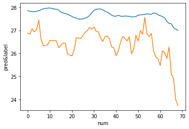

#模型保存
torch.save(lstm.state_dict(), "./stock.pth")


#重新加载模型，进行测试
model = Lstm(feature_size=feature_size,hidden_size=hidden_size,num_layers=num_layers)
model.load_state_dict(torch.load("./stock.pth"))
model.eval()

#读取测试数据
df_test = pd.read_csv('actual_data.csv')
print(df_test)

         date   open   high    low  close    volume
0  2021/11/29  24.06  24.13  23.67  23.83  33211134
1  2021/11/30  25.10  25.10  23.59  23.69  59059776
2   2021/12/1  25.03  25.33  24.76  25.14  30491050
3   2021/12/2  25.69  25.70  24.97  25.23  43458444
4   2021/12/3  25.01  26.38  24.76  25.70  78908600
5   2021/12/4  24.64  24.88  24.46  24.65  26092200
6   2021/12/5  25.01  25.22  24.53  24.64  48458572
7   2021/12/6  24.86  25.06  24.65  24.77  46163464
8   2021/12/7  24.28  25.05  24.19  24.85  39757868
9   2021/12/8  23.43  24.52  23.35  24.16  43993724

X_test = df_test.loc[df_test['close'].notnull(),df_test.columns[1:]]
Y_test = df_test.loc[df_test['close'].notnull(),df_test.columns[-2]]
X_test = X_test[:9].to_numpy().astype(np.float32)
Y_test = Y_test[9:].to_numpy().astype(np.float32)
X_test = np.expand_dims((X_test-mean_X)/std_X,0)
print(X_test, Y_test)

[[[-1.4159937  -1.4235495  -1.4362141  -1.4339249  -0.84247094]
  [-1.3457464  -1.358999   -1.4371747  -1.438578   -0.11689322]
  [-1.3460472  -1.3406453  -1.3569758  -1.3424493  -0.91625774]
  [-1.3001059  -1.3136134  -1.3390524  -1.3327416  -0.5548063 ]
  [-1.3392715  -1.2674377  -1.3485703  -1.2989068   0.43764323]
  [-1.3584667  -1.3566296  -1.3637093  -1.3614955  -1.0386132 ]
  [-1.3308277  -1.3313277  -1.3549037  -1.3579053  -0.41640592]
  [-1.3358696  -1.3369921  -1.3427285  -1.3454323  -0.47950524]
  [-1.3679413  -1.3332245  -1.3677566  -1.3359128  -0.6569169 ]]] [24.16]

out= model(torch.from_numpy(X_test)).detach().numpy()
out = out*std_Y+mean_Y
print("2012.12.8预测值：{},真实标签：{}".format(out, Y_test[0]))

2012.12.8预测值：26.66297721862793,真实标签：24.15999984741211

代码和数据链接：

https://download.csdn.net/download/qq_14845119/90461048