Frenet坐标系相关知识系统学习

---

零、Frenet坐标系简介 

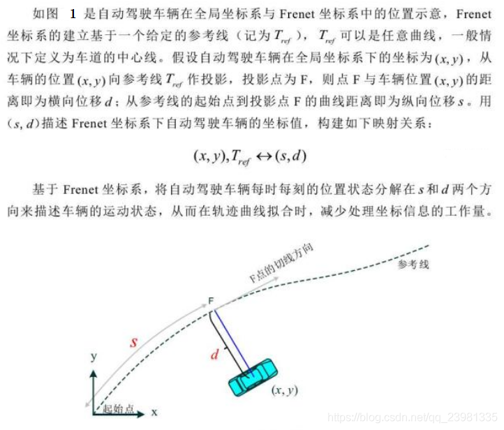
       自动驾驶汽车路径规划技术的难点之一在于规划过程中难以表达车辆与道路之间的相对位置,导致二者之间的相对关系不明确。因此,传统规划算法在笛卡尔坐标系下规划出的路径对于开放道路有良好的效果，但是对于公路环境，忽略车道信息导致路径的自由度太高而容易违反道路交通规则。在DAPRA汽车挑战赛期间，由斯坦福大学提出的路径规划算法将横向偏移(lateral offset)定义为相对于基础路径(baseframe)的垂直距离。由于基础路径为道路中心线,这样的定义方式使得道路与车辆之间的关系更为直观。

---

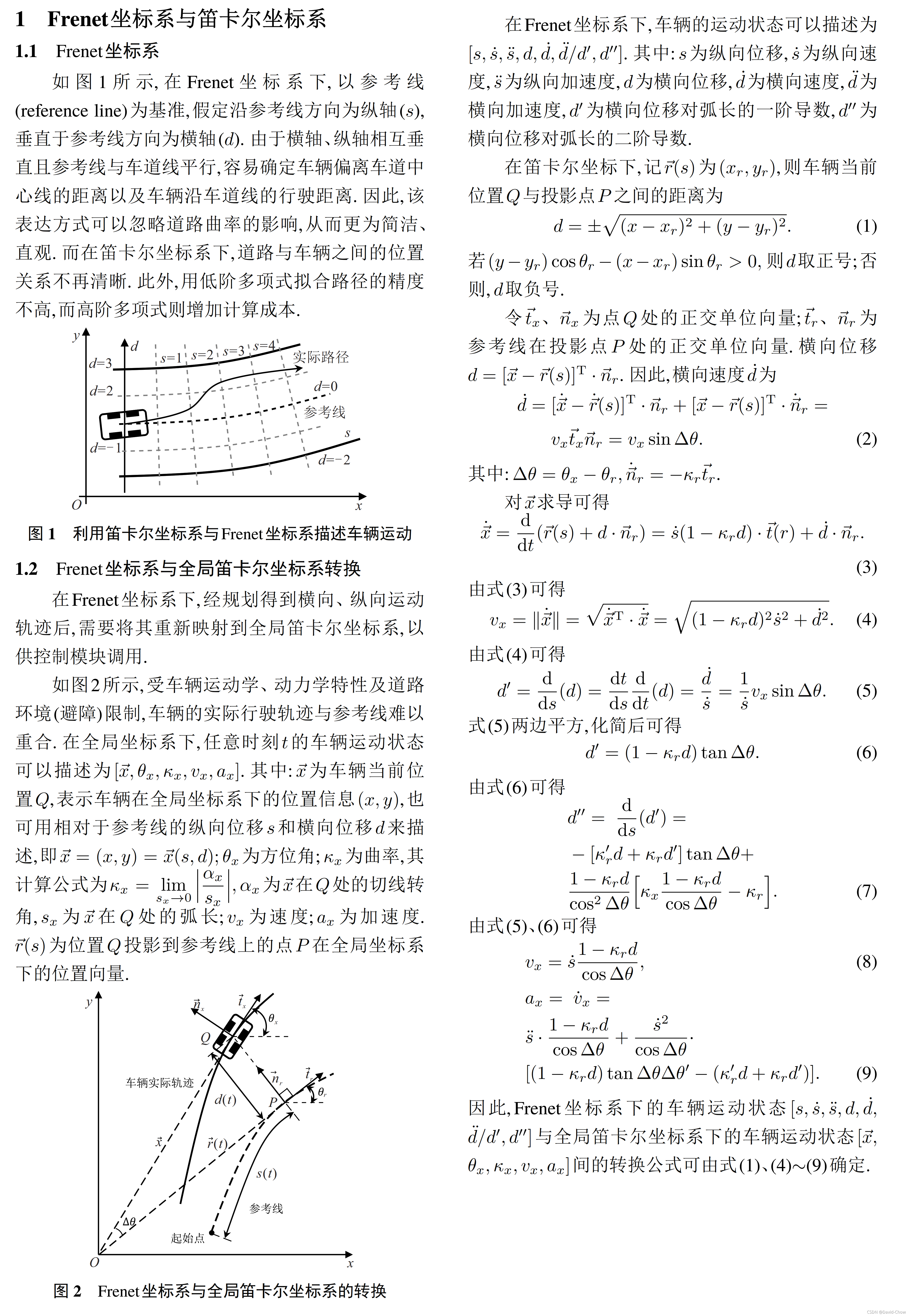
一、Frenet坐标系与全局坐标系的转换

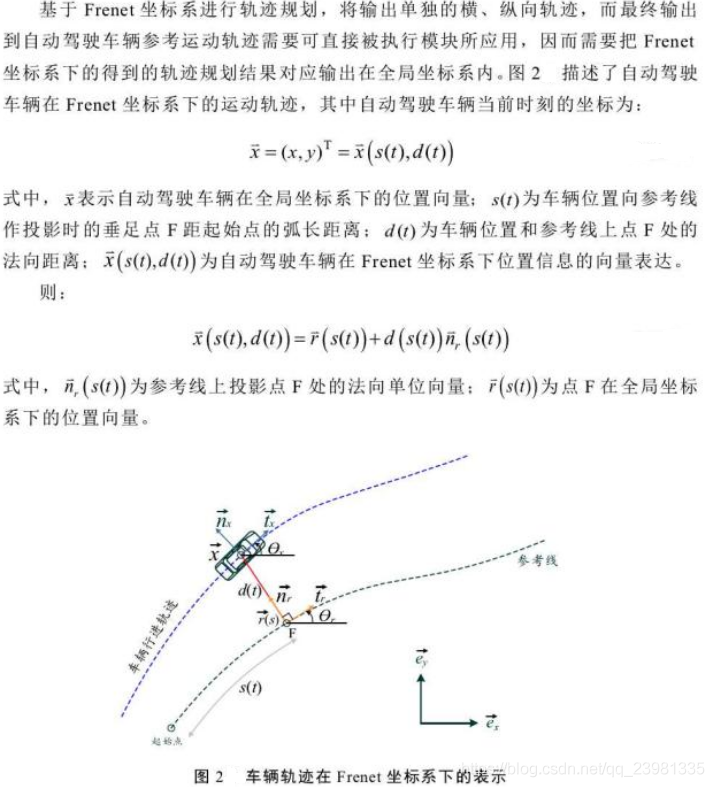
 Frenet坐标转化公式推导（Frenet 坐标系与全局笛卡尔坐标系转换）参考博客《轨迹规划1：Frenet坐标转化公式推导》

总结如下：

---

（1）《无人驾驶汽车系统入门（二十一）——基于Frenet优化轨迹的无人车动作规划方法》

（2）《控制及决策》期刊2021论文《基于Frenet坐标系的自动驾驶轨迹规划与优化算法》

二、基于jerk 的实时（横纵向）轨迹规划求解

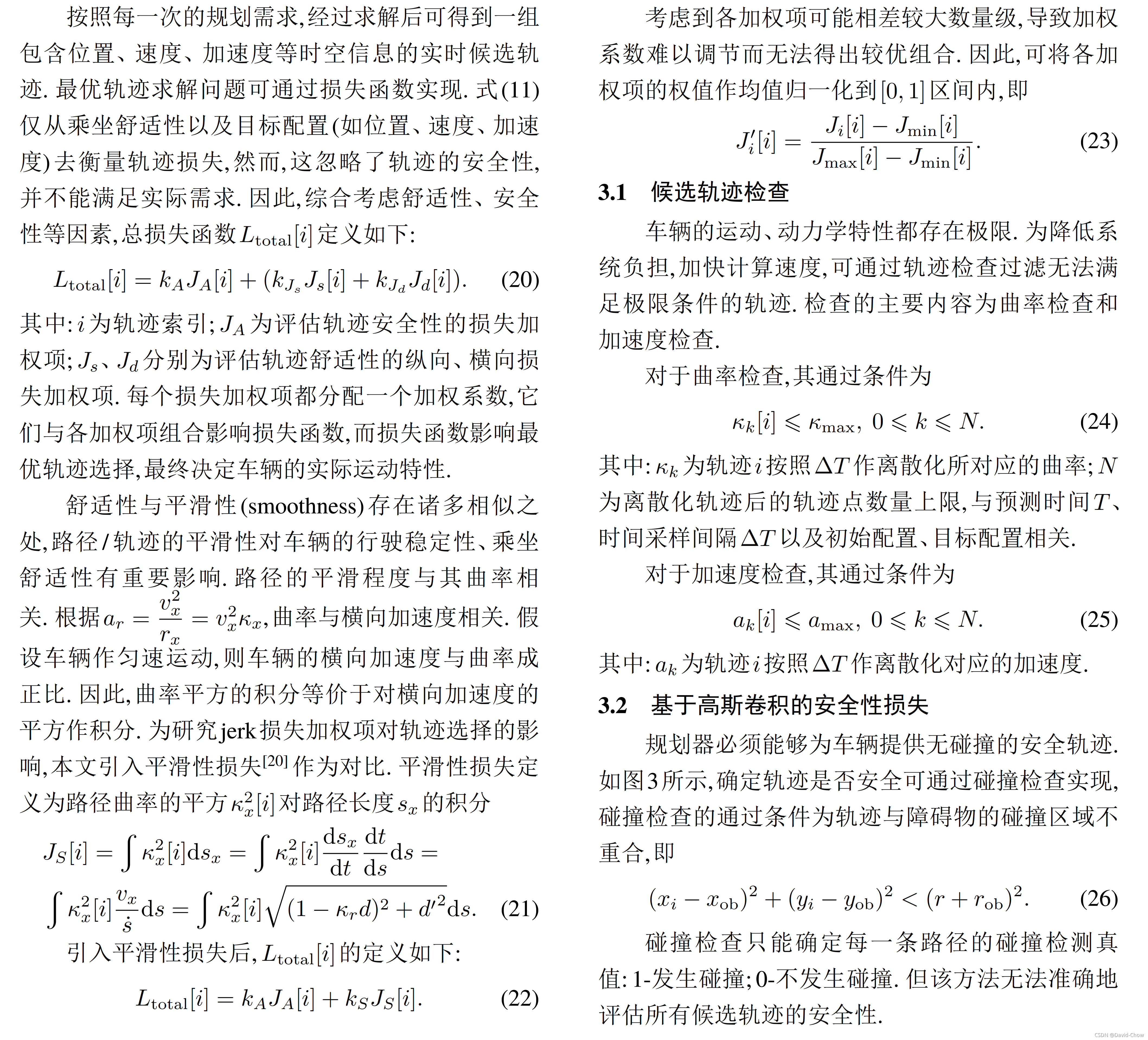
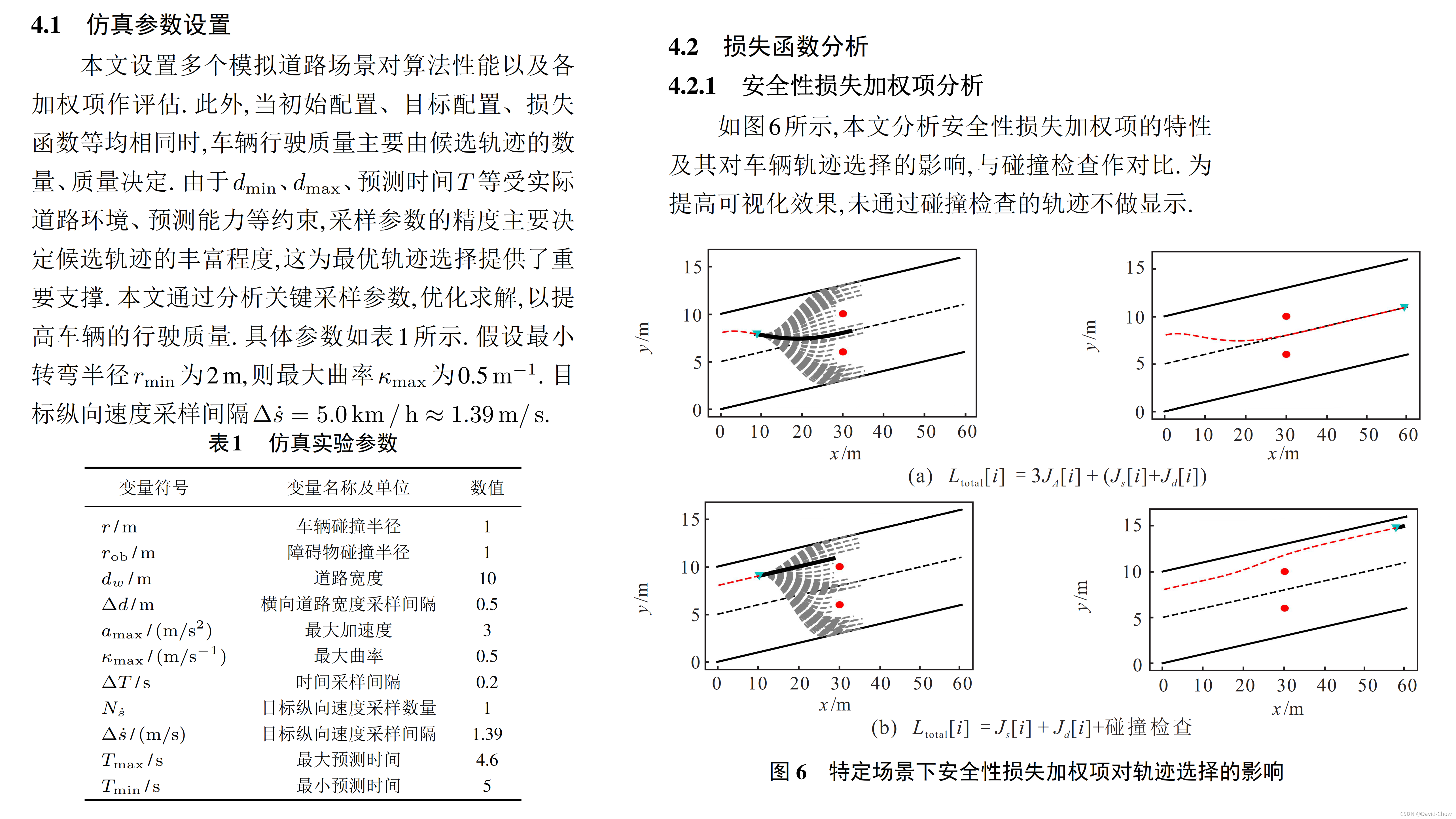
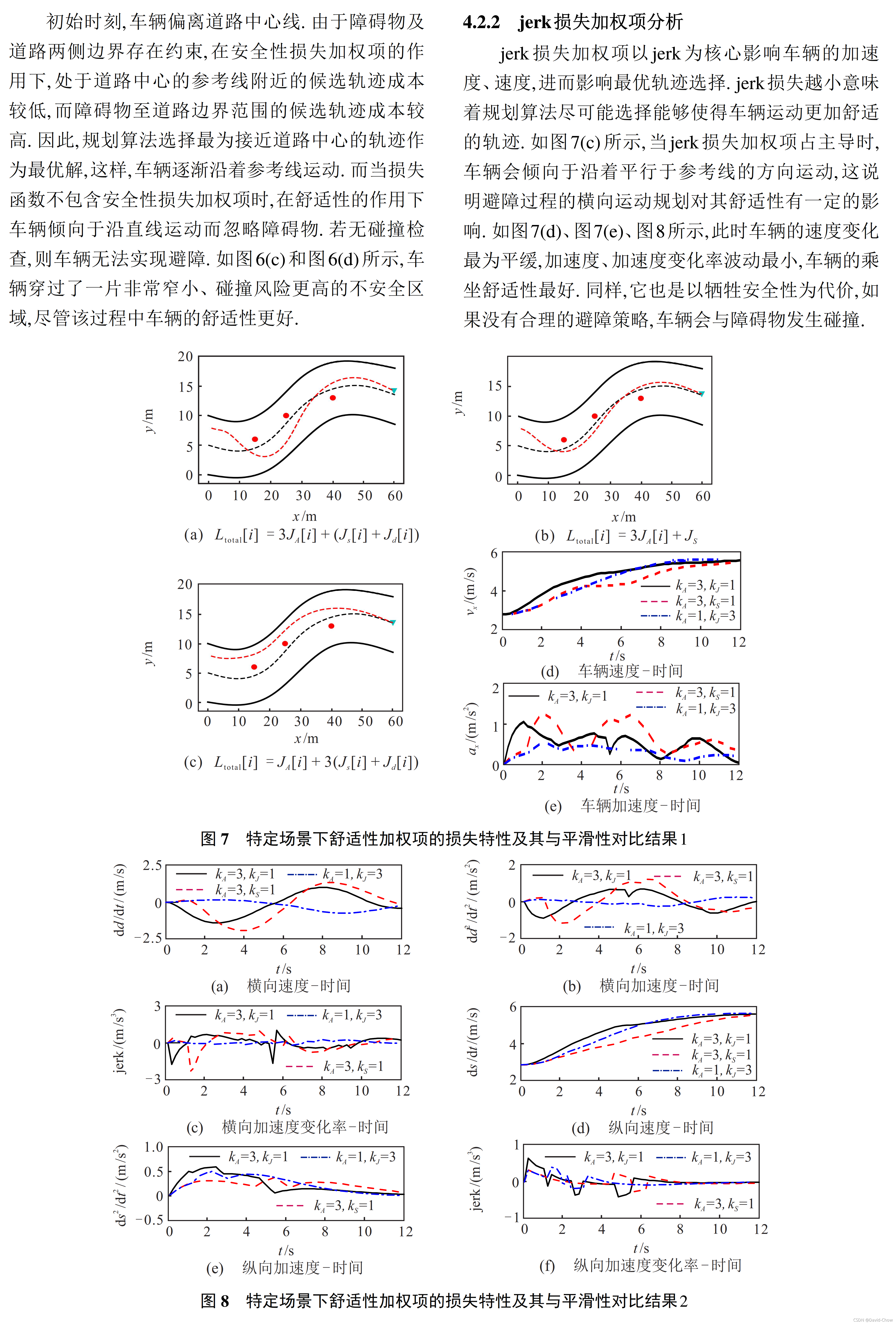
       可以基于Frenet坐标系，报据自动驾驶车辆的始末状态，利用五次多项式建立自动驾驶车辆轨迹规划模型，并建立各个场景下的轨迹质量评估函数。 基于Frenet坐标系，提出一种能够面向公路场景的轨迹规划算法。首先，利用Frenet坐标系，将二维的车辆运动解耦成相互独立的一维纵向、横向运动，构建以 jerk 为核心的一维独立积分系统，利用5次、4次多项式分别求解得到有限的横向、纵向集合；然后，基于高斯卷积、加速度变化率，从安全性和舒适性设计损失函数以最小化轨迹成本；最后，通过模拟类公路场景验证算法性能，并开展轨迹优化选择以及采样优化等内容的研究。研究结果表明，该算法为车辆规划出的轨迹平滑、舒适、安全性更高。

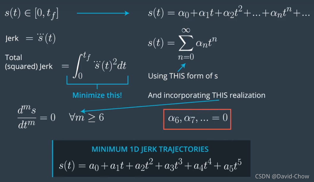
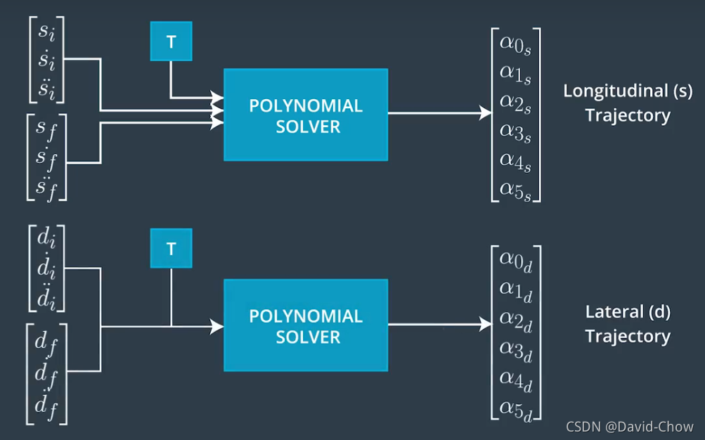
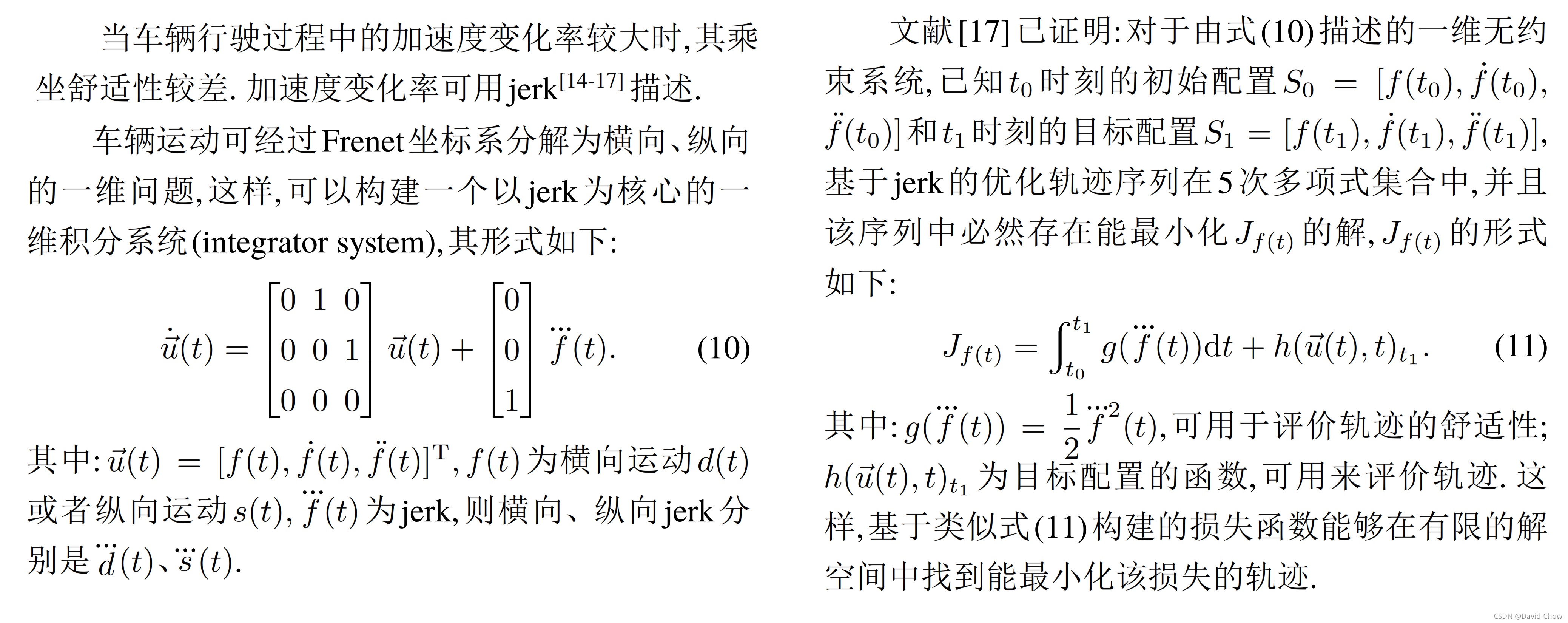
2.1 基于jerk 的一维无约束积分系统

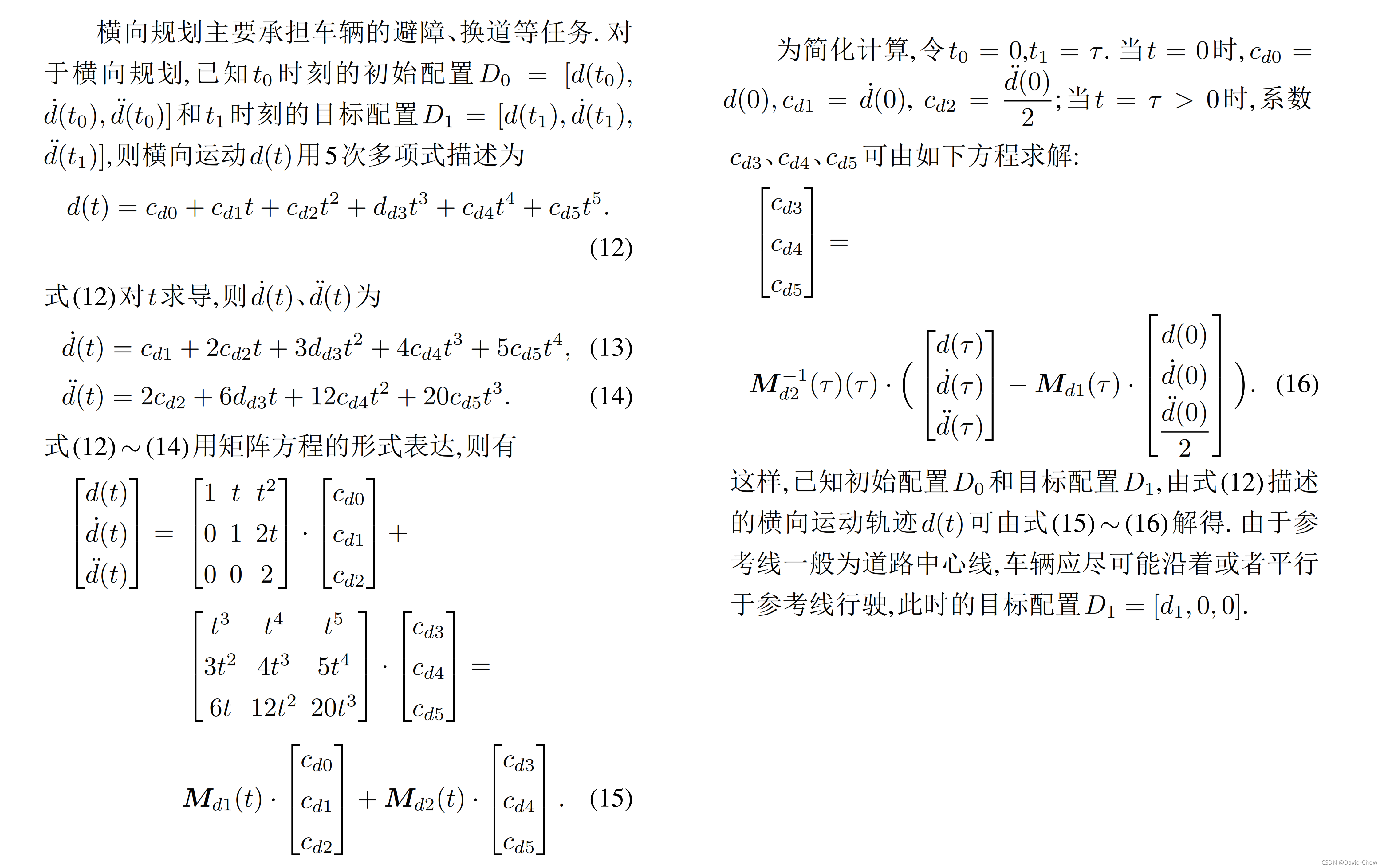
2.2 横向轨迹规划求解

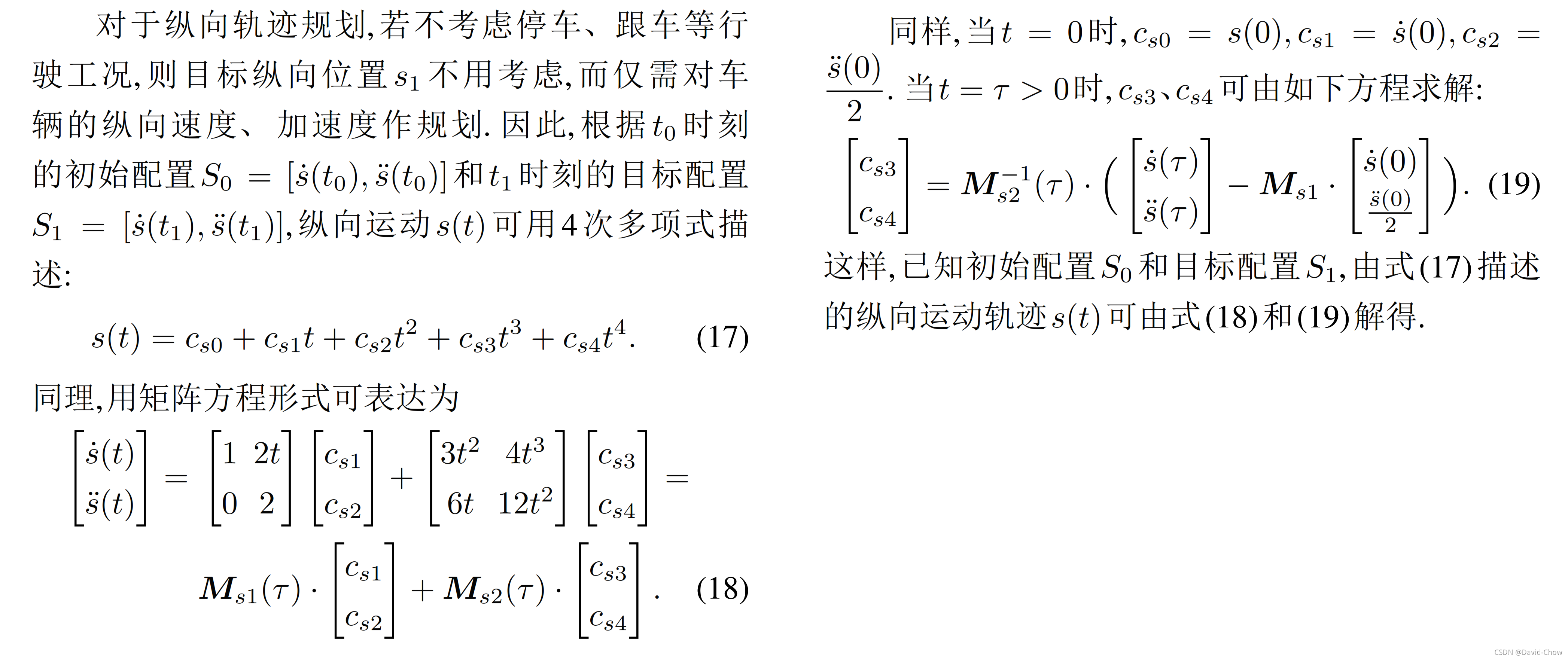
  2.3 纵向轨迹规划求解

三、 轨迹规划与最优选择

注意：

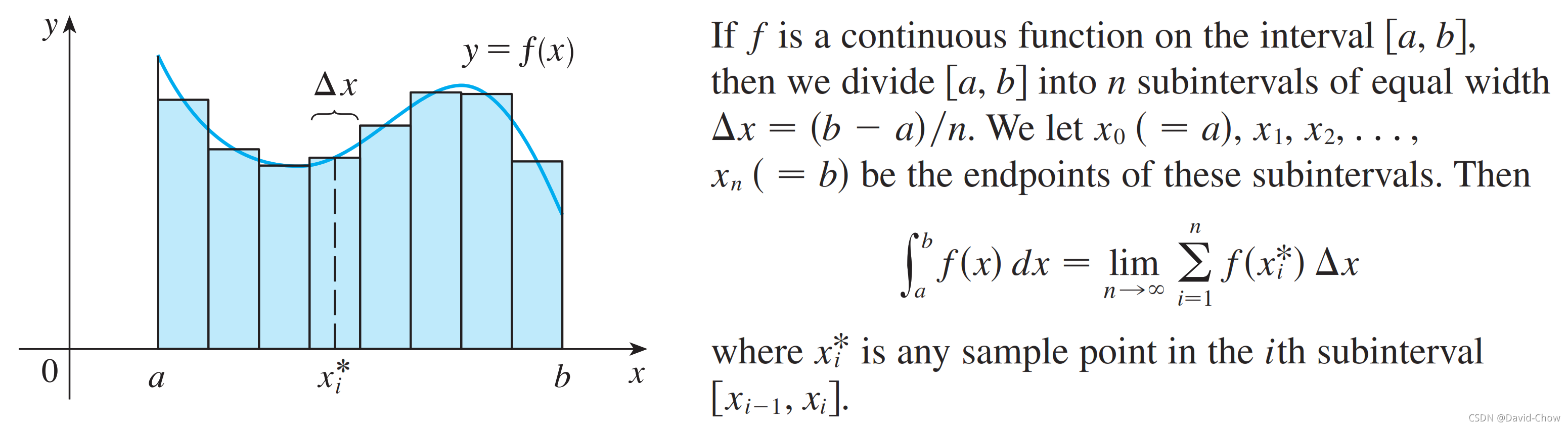
     在实际编码过程中，基于Jerk最小化的损失函数中的积分计算通过分割采样取点，将积分转换成黎曼和的形式进行计算，具体原理如下： 

 

四、 仿真评价与分析

 

 

 

---

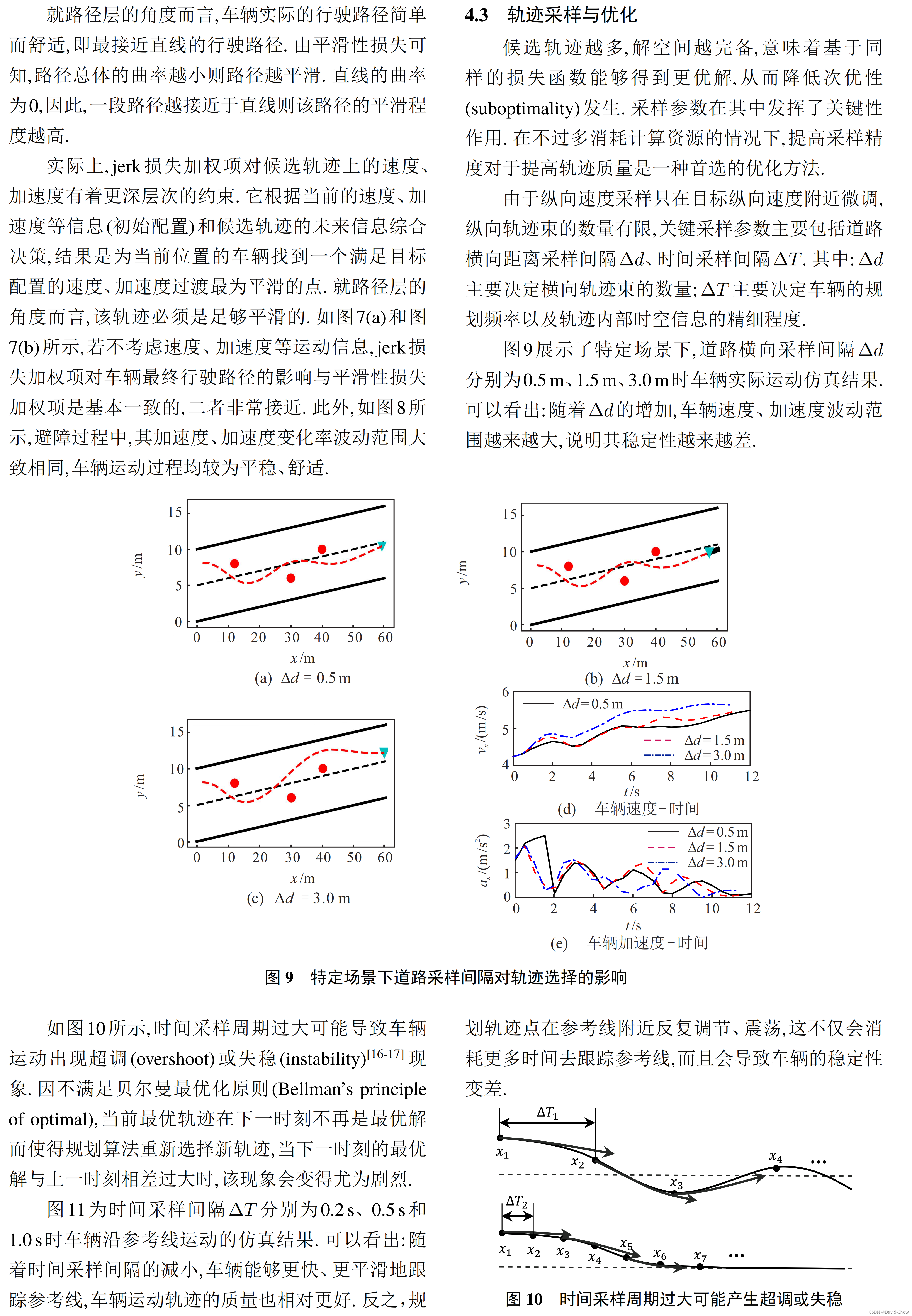
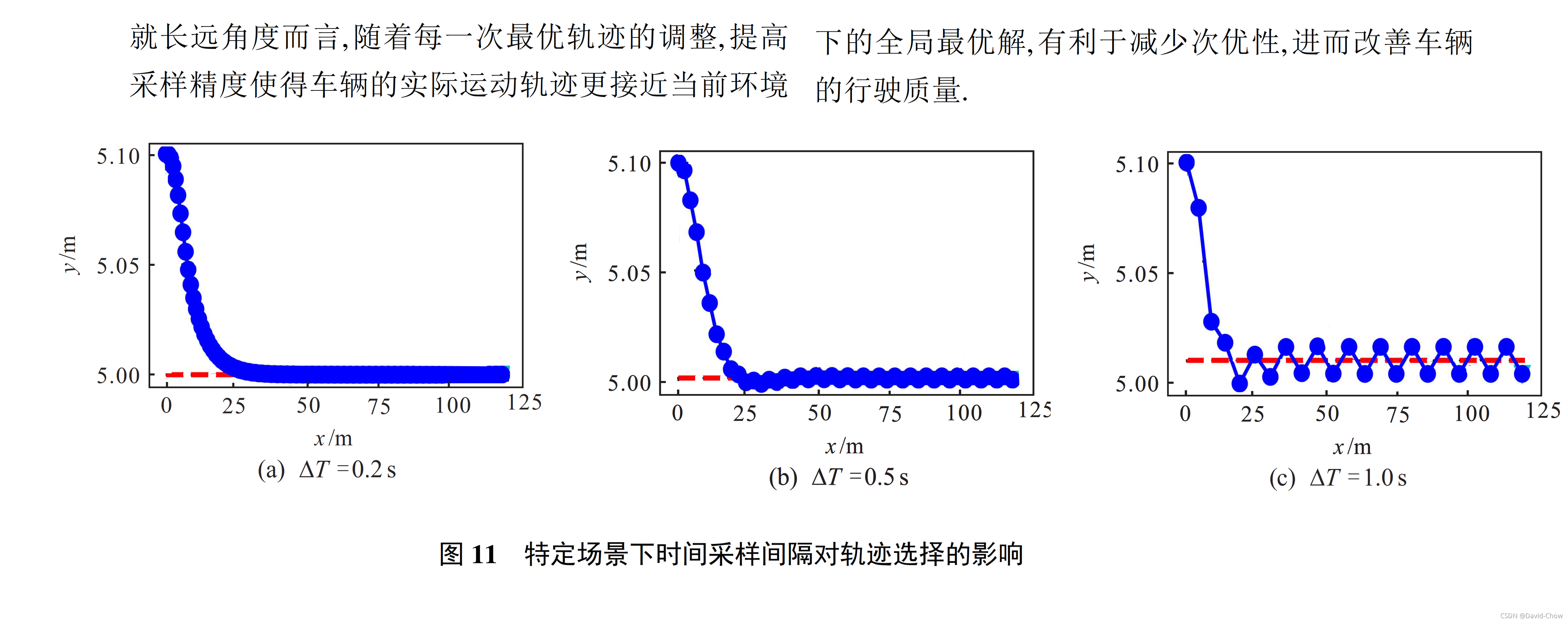
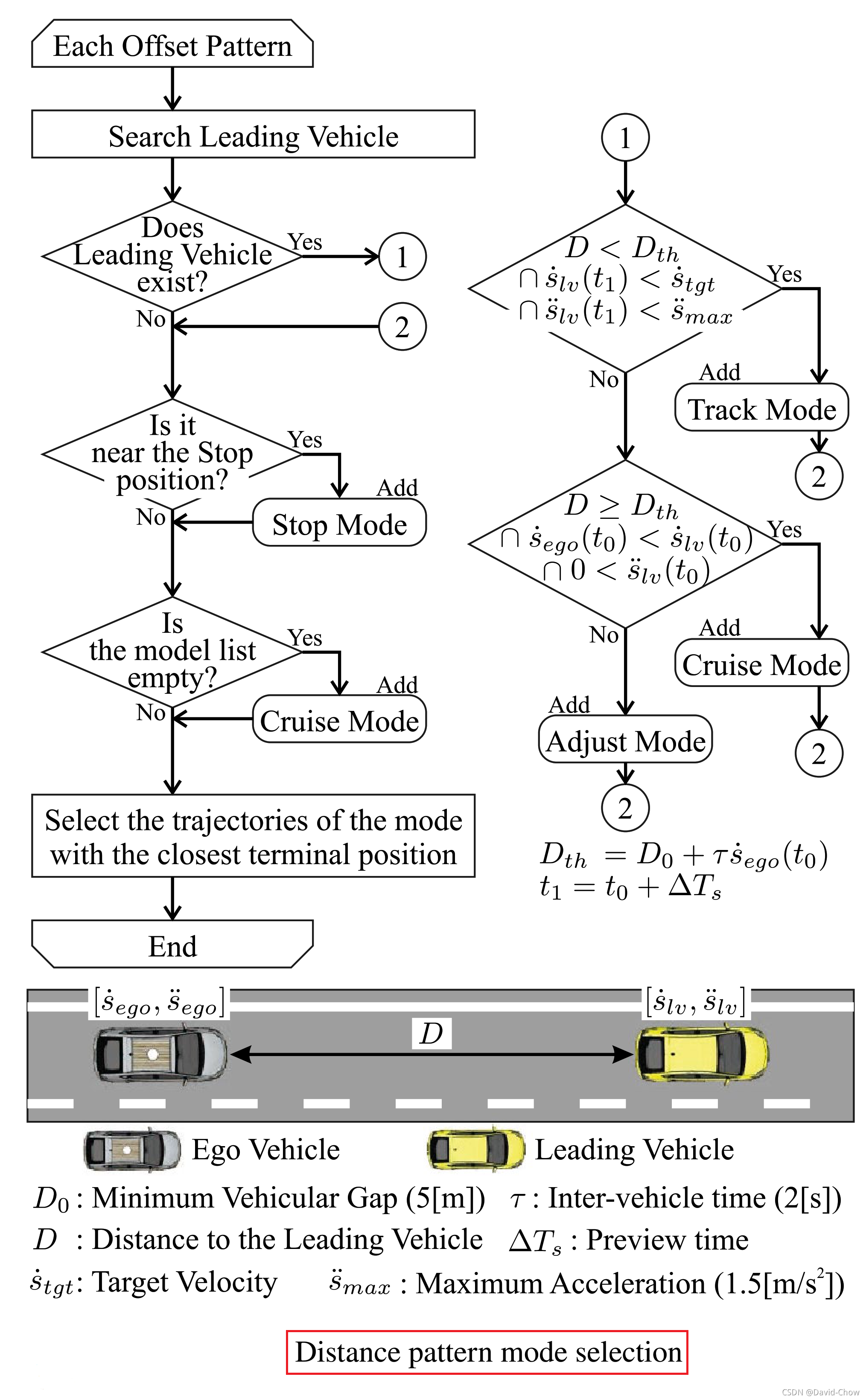
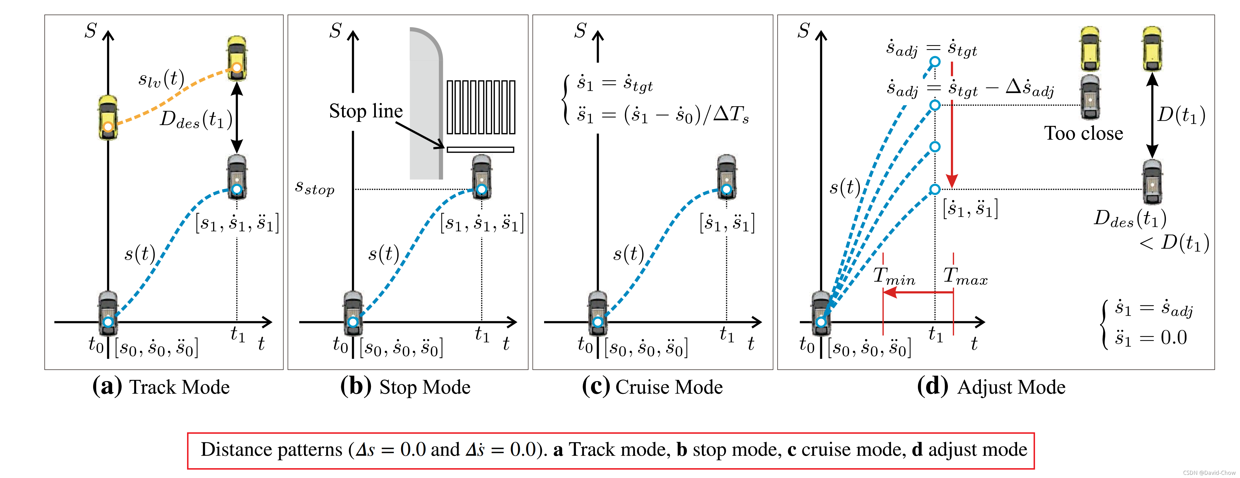
五、Distance Pattern行驶工况(包括速度保持、距离保持)下基于场景选择的轨迹生成

参见论文：《Trajectory optimization and state selection for urban automated driving》2018

基于模式选择的轨迹生成流程

各工况说明

---

六、深入学习

《Robotics-Path-Planning-04-Quintic-Polynomial-Solver》Github

《硕士论文-基于Frenet坐标系采样的自动驾驶轨迹规划算法研究》

《Optimal Trajectory Generation for Dynamic Street Scenarios in a Frene´t Frame》

《无人驾驶汽车系统入门（二十一）——基于Frenet优化轨迹的无人车动作规划方法》

《Apollo项目坐标系研究》

《第三期 预测——Frenet 坐标》

维基百科：Frenet–Serret formulas

---

七、代码学习

Trajectory Planning in the Frenet Space

------基于论文《Optimal Trajectory Generation for Dynamic Street Scenarios in a Frene´t Frame》

链接：Trajectory Planning in the Frenet Space - fjp.github.io 

代码

'''
https://fjp.at/posts/optimal-frenet/
http://fileadmin.cs.lth.se/ai/Proceedings/ICRA2010/MainConference/data/papers/1650.pdf
https://blog.csdn.net/AdamShan/article/details/80779615
'''
import pdb

import time
import pylab as pl
from IPython import display

import matplotlib
import numpy as np
import matplotlib.pyplot as plt

import copy
import math

from cubic_spline_planner import *


class quintic_polynomial:
    def __init__(self, xs, vxs, axs, xe, vxe, axe, T):
        # calc coefficient of quintic polynomial
        self.xs = xs
        self.vxs = vxs
        self.axs = axs
        self.xe = xe
        self.vxe = vxe
        self.axe = axe

        self.a0 = xs
        self.a1 = vxs
        self.a2 = axs / 2.0

        A = np.array([[T ** 3, T ** 4, T ** 5],
                      [3 * T ** 2, 4 * T ** 3, 5 * T ** 4],
                      [6 * T, 12 * T ** 2, 20 * T ** 3]])
        b = np.array([xe - self.a0 - self.a1 * T - self.a2 * T ** 2,
                      vxe - self.a1 - 2 * self.a2 * T,
                      axe - 2 * self.a2])
        x = np.linalg.solve(A, b)

        self.a3 = x[0]
        self.a4 = x[1]
        self.a5 = x[2]

    def calc_point(self, t):
        xt = self.a0 + self.a1 * t + self.a2 * t ** 2 + \
             self.a3 * t ** 3 + self.a4 * t ** 4 + self.a5 * t ** 5

        return xt

    def calc_first_derivative(self, t):
        xt = self.a1 + 2 * self.a2 * t + \
             3 * self.a3 * t ** 2 + 4 * self.a4 * t ** 3 + 5 * self.a5 * t ** 4

        return xt

    def calc_second_derivative(self, t):
        xt = 2 * self.a2 + 6 * self.a3 * t + 12 * self.a4 * t ** 2 + 20 * self.a5 * t ** 3

        return xt

    def calc_third_derivative(self, t):
        xt = 6 * self.a3 + 24 * self.a4 * t + 60 * self.a5 * t ** 2

        return xt


class quartic_polynomial:
    def __init__(self, xs, vxs, axs, vxe, axe, T):
        # calc coefficient of quintic polynomial
        self.xs = xs
        self.vxs = vxs
        self.axs = axs
        self.vxe = vxe
        self.axe = axe

        self.a0 = xs
        self.a1 = vxs
        self.a2 = axs / 2.0

        A = np.array([[3 * T ** 2, 4 * T ** 3],
                      [6 * T, 12 * T ** 2]])
        b = np.array([vxe - self.a1 - 2 * self.a2 * T,
                      axe - 2 * self.a2])
        x = np.linalg.solve(A, b)

        self.a3 = x[0]
        self.a4 = x[1]

    def calc_point(self, t):
        xt = self.a0 + self.a1 * t + self.a2 * t ** 2 + \
             self.a3 * t ** 3 + self.a4 * t ** 4

        return xt

    def calc_first_derivative(self, t):
        xt = self.a1 + 2 * self.a2 * t + \
             3 * self.a3 * t ** 2 + 4 * self.a4 * t ** 3

        return xt

    def calc_second_derivative(self, t):
        xt = 2 * self.a2 + 6 * self.a3 * t + 12 * self.a4 * t ** 2

        return xt

    def calc_third_derivative(self, t):
        xt = 6 * self.a3 + 24 * self.a4 * t

        return xt


class Frenet_path:
    def __init__(self):
        self.t = []
        self.d = []
        self.d_d = []
        self.d_dd = []
        self.d_ddd = []
        self.s = []
        self.s_d = []
        self.s_dd = []
        self.s_ddd = []
        self.cd = 0.0
        self.cv = 0.0
        self.cf = 0.0

        self.x = []
        self.y = []
        self.yaw = []
        self.ds = []
        self.c = []


# Parameter
MAX_SPEED = 50.0 / 3.6  # maximum speed [m/s]
MAX_ACCEL = 2.0  # maximum acceleration [m/ss]
MAX_CURVATURE = 1.0  # maximum curvature [1/m]
MAX_ROAD_WIDTH = 7.0  # maximum road width [m]
D_ROAD_W = 1.0  # road width sampling length [m]
DT = 0.2  # time tick [s]
MAXT = 5.0  # max prediction time [s]
MINT = 4.0  # min prediction time [s]
TARGET_SPEED = 30.0 / 3.6  # target speed [m/s]
D_T_S = 5.0 / 3.6  # target speed sampling length [m/s]
N_S_SAMPLE = 1  # sampling number of target speed
ROBOT_RADIUS = 2.0  # robot radius [m]

# cost weights
KJ = 0.1
KT = 0.1
KD = 1.0
KLAT = 1.0
KLON = 1.0


def calc_frenet_paths(c_speed, c_d, c_d_d, c_d_dd, s0):
    frenet_paths = []

    # generate path to each offset goal
    for di in np.arange(-MAX_ROAD_WIDTH, MAX_ROAD_WIDTH, D_ROAD_W):

        # Lateral motion planning
        for Ti in np.arange(MINT, MAXT, DT):
            print('di={0},Ti={1}'.format(di,Ti))
            fp = Frenet_path()

            lat_qp = quintic_polynomial(c_d, c_d_d, c_d_dd, di, 0.0, 0.0, Ti)

            fp.t = [t for t in np.arange(0.0, Ti, DT)] //通过取样分割，便于后面将0-Ti的积分转换为黎曼和（即每个分割点处的值之和）
            fp.d = [lat_qp.calc_point(t) for t in fp.t]
            fp.d_d = [lat_qp.calc_first_derivative(t) for t in fp.t]
            fp.d_dd = [lat_qp.calc_second_derivative(t) for t in fp.t]
            fp.d_ddd = [lat_qp.calc_third_derivative(t) for t in fp.t]

            # Loongitudinal motion planning (Velocity keeping)
            for tv in np.arange(TARGET_SPEED - D_T_S * N_S_SAMPLE, TARGET_SPEED + D_T_S * N_S_SAMPLE, D_T_S):
                tfp = copy.deepcopy(fp) #not tfp=fp

                lon_qp = quartic_polynomial(s0, c_speed, 0.0, tv, 0.0, Ti)

                tfp.s = [lon_qp.calc_point(t) for t in fp.t]
                tfp.s_d = [lon_qp.calc_first_derivative(t) for t in fp.t]
                tfp.s_dd = [lon_qp.calc_second_derivative(t) for t in fp.t]
                tfp.s_ddd = [lon_qp.calc_third_derivative(t) for t in fp.t]

                Jp = sum(np.power(tfp.d_ddd, 2))  # square of jerk ,the set T is discretized, and the integral is replaced with a summation
                Js = sum(np.power(tfp.s_ddd, 2))  # square of jerk,the set T is discretized, and the integral is replaced with a summation

                # square of diff from target speed
                ds = (TARGET_SPEED - tfp.s_d[-1]) ** 2

                tfp.cd = KJ * Jp + KT * Ti + KD * tfp.d[-1] ** 2
                tfp.cv = KJ * Js + KT * Ti + KD * ds
                tfp.cf = KLAT * tfp.cd + KLON * tfp.cv

                frenet_paths.append(tfp)

    return frenet_paths


faTrajX = []
faTrajY = []


def calc_global_paths(fplist, csp):
    # faTrajX = []
    # faTrajY = []

    for fp in fplist:

        # calc global positions
        for i in range(len(fp.s)):
            ix, iy = csp.calc_position(fp.s[i])
            if ix is None:
                break
            iyaw = csp.calc_yaw(fp.s[i])
            di = fp.d[i]
            fx = ix + di * math.cos(iyaw + math.pi / 2.0)
            fy = iy + di * math.sin(iyaw + math.pi / 2.0)
            fp.x.append(fx)
            fp.y.append(fy)

        # Just for plotting
        faTrajX.append(fp.x)
        faTrajY.append(fp.y)

        # calc yaw and ds
        for i in range(len(fp.x) - 1):
            dx = fp.x[i + 1] - fp.x[i]
            dy = fp.y[i + 1] - fp.y[i]
            fp.yaw.append(math.atan2(dy, dx))
            fp.ds.append(math.sqrt(dx ** 2 + dy ** 2))

        fp.yaw.append(fp.yaw[-1])
        fp.ds.append(fp.ds[-1])

        # calc curvature
        for i in range(len(fp.yaw) - 1):
            fp.c.append((fp.yaw[i + 1] - fp.yaw[i]) / fp.ds[i])

    return fplist


faTrajCollisionX = []
faTrajCollisionY = []
faObCollisionX = []
faObCollisionY = []


def check_collision(fp, ob):
    # pdb.set_trace()
    for i in range(len(ob[:, 0])):
        # Calculate the distance for each trajectory point to the current object
        d = [((ix - ob[i, 0]) ** 2 + (iy - ob[i, 1]) ** 2)
             for (ix, iy) in zip(fp.x, fp.y)]

        # Check if any trajectory point is too close to the object using the robot radius
        collision = any([di <= ROBOT_RADIUS ** 2 for di in d])

        if collision:
            # plot(ft.x, ft.y, 'rx')
            faTrajCollisionX.append(fp.x)
            faTrajCollisionY.append(fp.y)

            # plot(ox, oy, 'yo');
            # pdb.set_trace()
            if ob[i, 0] not in faObCollisionX or ob[i, 1] not in faObCollisionY:
                faObCollisionX.append(ob[i, 0])
                faObCollisionY.append(ob[i, 1])

            return True

    return False


# faTrajOkX = []
# faTrajOkY = []

def check_paths(fplist, ob):
    okind = []
    for i in range(len(fplist)):
        if any([v > MAX_SPEED for v in fplist[i].s_d]):  # Max speed check
            continue
        elif any([abs(a) > MAX_ACCEL for a in fplist[i].s_dd]):  # Max accel check
            continue
        elif any([abs(c) > MAX_CURVATURE for c in fplist[i].c]):  # Max curvature check
            continue
        elif check_collision(fplist[i], ob):
            continue

        okind.append(i)

    return [fplist[i] for i in okind]


fpplist = []


def frenet_optimal_planning(csp, s0, c_speed, c_d, c_d_d, c_d_dd, ob):
    # pdb.set_trace()
    fplist = calc_frenet_paths(c_speed, c_d, c_d_d, c_d_dd, s0)
    fplist = calc_global_paths(fplist, csp)
    fplist = check_paths(fplist, ob)



    # fpplist = deepcopy(fplist)
    fpplist.extend(fplist)

    # find minimum cost path
    mincost = float("inf")
    bestpath = None
    for fp in fplist:
        if mincost >= fp.cf:
            mincost = fp.cf
            bestpath = fp

    return bestpath


from cubic_spline_planner import *


def generate_target_course(x, y):
    csp = Spline2D(x, y)
    s = np.arange(0, csp.s[-1], 0.1)

    rx, ry, ryaw, rk = [], [], [], []
    for i_s in s:
        ix, iy = csp.calc_position(i_s)
        rx.append(ix)
        ry.append(iy)
        ryaw.append(csp.calc_yaw(i_s))
        rk.append(csp.calc_curvature(i_s))

    return rx, ry, ryaw, rk, csp


show_animation = True
# show_animation = False
# way points
wx = [0.0, 10.0, 20.5, 35.0, 70.5]
wy = [0.0, -6.0, 5.0, 6.5, 0.0]
# obstacle lists
ob = np.array([[20.0, 10.0],
               [30.0, 6.0],
               [30.0, 8.0],
               [35.0, 8.0],
               [50.0, 3.0]
               ])

tx, ty, tyaw, tc, csp = generate_target_course(wx, wy)


# initial state
c_speed = 10.0 / 3.6  # current speed [m/s]
c_d = 2.0  # current lateral position [m]
c_d_d = 0.0  # current lateral speed [m/s]
c_d_dd = 0.0  # current latral acceleration [m/s]
s0 = 0.0  # current course position

area = 20.0  # animation area length [m]

fig = plt.figure()
plt.ion()

faTx = tx
faTy = ty
faObx = ob[:, 0]
faOby = ob[:, 1]
faPathx = []
faPathy = []
faRobotx = []
faRoboty = []
faSpeed = []
for i in range(100):
    path = frenet_optimal_planning(csp, s0, c_speed, c_d, c_d_d, c_d_dd, ob)
    s0 = path.s[1]
    c_d = path.d[1]
    c_d_d = path.d_d[1]
    c_d_dd = path.d_dd[1]
    c_speed = path.s_d[1]

    if np.hypot(path.x[1] - tx[-1], path.y[1] - ty[-1]) <= 1.0:
        print("Goal")
        break

    faPathx.append(path.x[1:])
    faPathy.append(path.y[1:])
    faRobotx.append(path.x[1])
    faRoboty.append(path.y[1])
    faSpeed.append(c_speed)
    if show_animation:
        plt.cla()
        plt.plot(tx, ty, animated=True)
        plt.plot(ob[:, 0], ob[:, 1], "xk")
        plt.plot(tx,ty,'-',color='crimson')

        plt.plot(path.x[1], path.y[1], "vc")

        for (ix, iy) in zip(faTrajX, faTrajY):
            # pdb.set_trace()
            plt.plot(ix[1:], iy[1:], '-', color=[0.5, 0.5, 0.5])


        faTrajX = []
        faTrajY = []

        for (ix, iy) in zip(faTrajCollisionX, faTrajCollisionY):
            # pdb.set_trace()
            plt.plot(ix[1:], iy[1:], 'rx')
        faTrajCollisionX = []
        faTrajCollisionY = []
        # pdb.set_trace()
        for fp in fpplist:
            # pdb.set_trace()
            plt.plot(fp.x[1:], fp.y[1:], '-g')
        fpplist = []

        # pdb.set_trace()
        for (ix, iy) in zip(faObCollisionX, faObCollisionY):
            # pdb.set_trace()
            plt.plot(ix, iy, 'oy')
        faObCollisionX = []
        faObCollisionY = []

        plt.plot(path.x[1:], path.y[1:], "-ob")
        print('len:{}'.format(len(path.x[1:])))

        plt.xlim(path.x[1] - area, path.x[-1] + area)
        plt.ylim(path.y[1] - area, path.y[-1] + area)
        plt.title("v[km/h]:" + str(c_speed * 3.6)[0:4])
        plt.grid(True)
        plt.pause(0.00001)
        plt.show()
        # display.clear_output(wait=True)
        # display.display(pl.gcf())
        plt.pause(0.1)
        print("Finish")


plt.ioff()

运行结果（片段）