GEE数据集——DynQual 全球地表水水质数据集

DynQual 全球地表水水质数据集
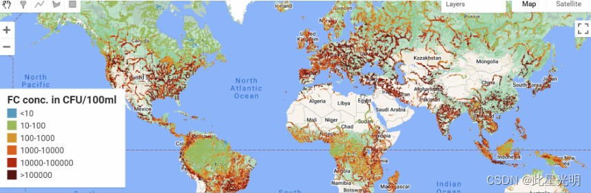
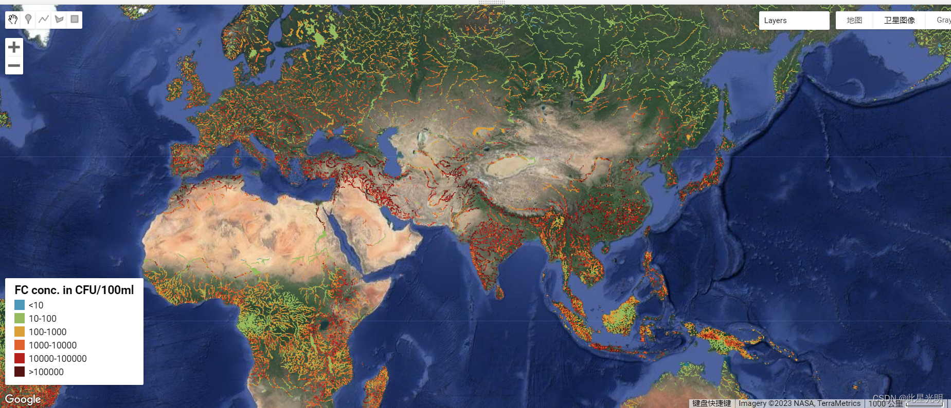
保持最佳地表水质对保护生态系统和确保人类安全用水至关重要。然而，我们对地表水质的了解主要依赖于监测站的数据，而这些数据在空间上是有限的，在时间上也是支离破碎的。针对这些局限性，我们引入了地表水质动态模型（DynQual）。该模型可模拟水温（Tw）以及总溶解固体（TDS）、生物需氧量（BOD）和粪大肠菌群（FC）的浓度。DynQual 以日为时间步长，空间分辨率为 5 弧分（∼ 10 千米）。前言 – 人工智能教程

这种全面的全球模型使我们能够根据现实世界的水质观测结果对其性能进行评估。此外，我们还介绍了 1980 年至 2019 年期间 TDS、BOD 和 FC 浓度的空间模式和时间趋势。我们的分析确定了造成地表水污染的主要行业。值得注意的是，DynQual 发现了广泛的多重污染热点，尤其是在印度北部和中国东部，尽管水质问题遍及全球所有地区。水质下降最严重的地区是发展中地区，尤其是撒哈拉以南非洲和南亚。研究人员可以访问开源模型代码（Jones 等人，2023 年）以及全球数据集，其中包括每月 5 弧分分辨率的模拟水文、Tw、TDS、BOD 和 FC（Jones 等人，2022 年 b）。这些数据集具有加强从生态研究到人类健康和水资源短缺评估等各种研究的潜力。欲了解更多信息，请访问 DynQual 模型代码UU-Hydro/DYNQUAL: DynQual v1.0 | Zenodo和全球地表水质数据集Global monthly hydrology and water quality datasets, derived from the dynamical surface water quality model (DynQual) at 10 km spatial resolution | Zenodo。您可在此阅读论文全文GMD - DynQual v1.0: a high-resolution global surface water quality model

请参阅原始论文中有关显示浓度图的指导，作者建议只在特定的排水量/渠道贮水量阈值以上绘制浓度图。

免责声明：数据集的全部或部分描述由作者或其作品提供。

数据集预处理
下载数据集，并将其从 NetCDF 转换为 Geotiff 格式，以便输入。由于这是一个多波段的月度汇总图像，而且我希望允许用户按时间段进行切分，因此图像波段作为单个图像进行了分离，总体结果是附有日期范围信息的图像集合。

引用Citation¶

Jones, E. R., Bierkens, M. F. P., Wanders, N., Sutanudjaja, E. H., van Beek, L. P. H., and van Vliet, M. T. H.:
DynQual v1.0: a high-resolution global surface water quality model, Geosci. Model Dev., 16, 4481–4500, https://doi.
org/10.5194/gmd-16-4481-2023, 2023.

数据引用Dataset citation¶

Jones, E. R., Bierkens, M. F. P., Wanders, N., Sutanudjaja, E. H., van Beek, L. P. H., & van Vliet, M. T. H.
(2022). Global monthly hydrology and water quality datasets, derived from the dynamical surface water quality
model (DynQual) at 10 km spatial resolution [Data set]. In Geoscientific Model Development (Vol. 16, pp.
4481–4500). Zenodo. https://doi.org/10.5281/zenodo.7139222

  

Earth Engine Snippet¶

var fc = ee.ImageCollection("projects/sat-io/open-datasets/DYNQUAL/fecal-coliform");
var discharge = ee.ImageCollection("projects/sat-io/open-datasets/DYNQUAL/discharge");
var tds = ee.ImageCollection("projects/sat-io/open-datasets/DYNQUAL/total-dissolved-solids");
var bod = ee.ImageCollection("projects/sat-io/open-datasets/DYNQUAL/biological-oxygen-demand");
var water_temp = ee.ImageCollection("projects/sat-io/open-datasets/DYNQUAL/water-temperature");

var discharge = ee.ImageCollection("projects/sat-io/open-datasets/DYNQUAL/discharge"),
    fc = ee.ImageCollection("projects/sat-io/open-datasets/DYNQUAL/fecal-coliform");
    var joinFilter = ee.Filter.equals({
  leftField: 'system:time_start',
  rightField: 'system:time_start'
});

// Define the join type
var joinType = 'inner';

// Join the image collections based on system:time_start
var joinedCollection = ee.Join.inner().apply({
  primary: fc,
  secondary: discharge,
  condition: joinFilter
});

print('Joined Collection:', joinedCollection);

var multibandCollection = joinedCollection.map(function(image) {
  var fc_band = ee.Image(image.get('primary'));
  var discharge_band = ee.Image(image.get('secondary'));

  // Merge the bands from both collections
  var multibandImage = fc_band.select('b1').rename('fc').addBands(discharge_band.select('b1').rename('discharge'));

  return multibandImage;
});
print(multibandCollection)
var conditional = function(image){
  var fc_masked = image.select('fc').mask(image.select('discharge').gt(10))
  return fc_masked
}

var fc_constrained = ee.ImageCollection(multibandCollection).map(conditional)

var popcount_intervals =
'<RasterSymbolizer>' +
' <ColorMap type="intervals" extended="false" >' +
    '<ColorMapEntry color="#4E99BB" quantity="0" label="No Data"/>' +
    '<ColorMapEntry color="#97BB5F" quantity="10" label="Population Count (Estimate)"/>' +
    '<ColorMapEntry color="#DBA03A" quantity="100" label="Population Count (Estimate)"/>' +
    '<ColorMapEntry color="#E1622D" quantity="1000" label="Population Count (Estimate)"/>' +
    '<ColorMapEntry color="#B51F1D" quantity="10000" label="Population Count (Estimate)"/>' +
    '<ColorMapEntry color="#531412" quantity="100000" label="Population Count (Estimate)"/>' +

  '</ColorMap>' +
'</RasterSymbolizer>';

// Define a dictionary which will be used to make legend and visualize image on map
//4E99BB,97BB5F,DBA03A,E1622D,B51F1D,531412
var dict = {
  "names": [
    "<10",
    "10-100",
    "100-1000",
    "1000-10000",
    "10000-100000",
    ">100000",
  ],
  "colors": [
    "#4E99BB",
    "#97BB5F",
    "#DBA03A",
    "#E1622D",
    "#B51F1D",
    "#531412",
  ]};
  
  // Create a panel to hold the legend widget
var legend = ui.Panel({
  style: {
    position: 'bottom-left',
    padding: '8px 15px'
  }
});

// Function to generate the legend
function addCategoricalLegend(panel, dict, title) {
  
  // Create and add the legend title.
  var legendTitle = ui.Label({
    value: title,
    style: {
      fontWeight: 'bold',
      fontSize: '18px',
      margin: '0 0 4px 0',
      padding: '0'
    }
  });
  panel.add(legendTitle);
  
  var loading = ui.Label('Loading legend...', {margin: '2px 0 4px 0'});
  panel.add(loading);
  
  // Creates and styles 1 row of the legend.
  var makeRow = function(color, name) {
    // Create the label that is actually the colored box.
    var colorBox = ui.Label({
      style: {
        backgroundColor: color,
        // Use padding to give the box height and width.
        padding: '8px',
        margin: '0 0 4px 0'
      }
    });
  
    // Create the label filled with the description text.
    var description = ui.Label({
      value: name,
      style: {margin: '0 0 4px 6px'}
    });
  
    return ui.Panel({
      widgets: [colorBox, description],
      layout: ui.Panel.Layout.Flow('horizontal')
    });
  };
  
  // Get the list of palette colors and class names from the image.
  var palette = dict['colors'];
  var names = dict['names'];
  loading.style().set('shown', false);
  
  for (var i = 0; i < names.length; i++) {
    panel.add(makeRow(palette[i], names[i]));
  }
  
  Map.add(panel);
}

addCategoricalLegend(legend, dict, 'FC conc. in CFU/100ml');
var snazzy = require("users/aazuspan/snazzy:styles");
snazzy.addStyle("https://snazzymaps.com/style/132/light-gray", "Grayscale");

Map.addLayer(fc_constrained.sort('system:time_start').first().sldStyle(popcount_intervals), {}, 'FC 1980-01-01');
Map.addLayer(fc_constrained.sort('system:time_start',false).first().sldStyle(popcount_intervals), {}, 'FC 2019-12-31');

 

代码链接Sample Code: https://code.earthengine.google.com/?scriptPath=users/sat-io/awesome-gee-catalog-examples:hydrology/DYNQUAL-EXAMPLE

License¶

Creative Commons Attribution 4.0 International Public License

Created by: Jones, E. R., Bierkens, M. F. P., Wanders, N., Sutanudjaja, E. H., van Beek, L. P. H., and van Vliet, M. T. H.

Curated in GEE by: Samapriya Roy

Keywords: water quality, discharge, water temperature, total dissolved solids, TDS, salinity, biological oxygen demand, BOD, fecal coliform, FC