非线性系统的反步法

  当被控对象含有未知参数时，通过设计李雅普诺夫函数使参数估计和被控对象的输出同时收敛。本文主要内容为，第一部分介绍使用李雅普诺夫法估计参数的基本原理，第二部分介绍参数不匹配情况下的反步法，第三部分对其中一个问题进行仿真。

参数估计

一阶系统参数估计

对被控对象 $y^{\prime }=a+bu$，$a$ 和 $b$ 均未知。写成矩阵形式
$$y^{\prime }={\theta }^{\ast \text{T}}\varphi =\left[\begin{array}{cc}a& b\end{array}\right]\left[\begin{array}{c}1\\ u\end{array}\right]$$
取 $u=\frac{1}{b}(-a-ky+k{y}_m+y_m^{\prime })$，则
$$\begin{array}{rl}& y^{\prime }=-ky+k{y}_m+y_m^{\prime }\\ & (y-y_m{)}^{\prime }=-k(y-y_m)\end{array}$$
$a,b$ 的估计值分别记作 $\hat{a},\hat{b}$，则 $y_m^{\prime }=\hat{b}u+\hat{a}+ky-k{y}_m$。
定义参数估计误差 $\tilde{\theta }(t)=\hat{\theta }(t)-{\theta }^{\ast }$ 和跟踪误差 $e=y-y_m$，则 ${\tilde{\theta }}^{\prime }(t)={\hat{\theta }}^{\prime }(t)$，
$$\begin{array}{rl}{e}^{\prime }(t)=& y^{\prime }-y_m^{\prime }\\ =& a+bu-(\hat{a}+\hat{b}u+ky-k{y}_m)\\ =& a-\hat{a}+(b-\hat{b})u-ke=-ke-{\tilde{\theta }}^{\text{T}}\varphi \end{array}$$
取候选李雅普诺夫函数
$$V(e,\tilde{\theta })=\frac{1}{2}{e}^2+\frac{1}{2}{\tilde{\theta }}^{\text{T}}\tilde{\theta }$$
则
$$\begin{array}{rl}{V}^{\prime }=& e{e}^{\prime }+{\tilde{\theta }}^{\text{T}}{\tilde{\theta }}^{\prime }\\ =& e(-ke-{\tilde{\theta }}^{\text{T}}\varphi )+{\tilde{\theta }}^{\text{T}}{\tilde{\theta }}^{\prime }\\ =& -k{e}^2+{\tilde{\theta }}^{\text{T}}({\hat{\theta }}^{\prime }-e\varphi )\end{array}$$
取 ${\hat{\theta }}^{\prime }=e\varphi$ 时可使得 $V$ 是李雅普诺夫函数，即
$$\begin{array}{rl}{\hat{a}}^{\prime }=& e\\ {\hat{b}}^{\prime }=& eu\end{array}$$

高阶系统参数估计

对被控对象
$$\begin{array}{rl}& x^{\prime }=Ax+Bu\\ & y=Cx\end{array}$$
$A,B,C$ 均未知。
注意到 $B,C$ 不可逆，对 $y$ 求导
$$y^{\prime }=C{x}^{\prime }=CAx+CBu$$
取 $\widehat{CA},\widehat{CB}$ 为待估计的参数，则取
$$u=\frac{1}{\widehat{CB}}\left[-\widehat{CA}x+y_m^{\prime }-K(y-y_m)\right]$$
当参数估计误差为0时，代入 $y$ 得
$$y^{\prime }-y_m^{\prime }=-K(y-y_m)$$
误差不为0时，$y_m^{\prime }=\widehat{CB}u+\widehat{CA}x+Ky-K{y}_m$。记
$$y^{\prime }={\theta }^{\ast \text{T}}\varphi =\left[\begin{array}{cc}CA& CB\end{array}\right]\left[\begin{array}{c}x\\ u\end{array}\right]$$
设 $\tilde{\theta }(t)=\hat{\theta }(t)-{\theta }^{\ast },e=y-y_m$，则
$$\begin{array}{rl}{e}^{\prime }(t)=& y^{\prime }-y_m^{\prime }\\ =& CAx+CBu-(\widehat{CB}u+\widehat{CA}x+Ky-K{y}_m)\\ =& (CA-\widehat{CA})x+(CB-\widehat{CB})u-ke=-ke-{\tilde{\theta }}^{\text{T}}\varphi \end{array}$$
取候选李雅普诺夫函数
$$V(e,\tilde{\theta })=\frac{1}{2}{e}^2+\frac{1}{2}{\tilde{\theta }}^{\text{T}}\tilde{\theta }$$
剩下步骤与一阶系统相同。

反步法

例1

$$x^{\prime }=\theta \varphi (x)+u$$
其中 $\theta$ 未知。取 $u=-\hat{\theta }\varphi (x)-kx$，候选李雅普诺夫函数
$$V(e,\tilde{\theta })=\frac{1}{2}{x}^2+\frac{1}{2}{\tilde{\theta }}^2$$
则
$$\begin{array}{rl}{V}^{\prime }=& x{x}^{\prime }+\tilde{\theta }{\tilde{\theta }}^{\prime }\\ =& x\theta \varphi +x(-\hat{\theta }\varphi -kx)+\tilde{\theta }{\tilde{\theta }}^{\prime }\\ =& -k{x}^2-x\varphi \tilde{\theta }+\tilde{\theta }{\tilde{\theta }}^{\prime }\end{array}$$
取 ${\tilde{\theta }}^{\prime }={\hat{\theta }}^{\prime }=x\varphi$，则 $V^{\prime }=-k{x}^2\le 0$。
  李雅普诺夫函数小于等于0不能保证收敛，需要证明。$V$ 单调下降有下界，所以 $V$ 的极限一定存在。
$$V(\infty )-V(0)=-k{\int }_0^{\infty }{x}^2\text{d}x,x\in L_2$$
$x$ 有界，$\tilde{\theta }$ 在 $V$ 中所以有界，所以 $u$ 有界，$x^{\prime }$ 有界，由信号收敛引理得 $x$ 极限存在。但是，除非充分激励，否则不能保证 $\hat{\theta }$ 收敛到 $\theta$。

例2

$$\begin{gathered} x_1^{\prime }={\varphi }_1(x_1)+x_2 \\ {x}_2^{\prime }=\theta {\varphi }_2(\vec{x})+u \end{gathered}$$
  $\theta$ 已知时，反馈线性化，令 $y=x_1$，则 $y^{\prime }=x_1^{\prime }=x_2+{\varphi }_1$，$y^{\prime \prime }=\theta {\varphi }_2+{\varphi }_1^{\prime }+u$。取 $u=-\theta {\varphi }_2-{\varphi }_1-k_1{y}^{\prime }-k_{2}y$，则 $y^{\prime \prime }=-k_1{y}^{\prime }-k_{2}y$。判断
$$T(x)=\left[\begin{array}{c}y\\ y^{\prime }\end{array}\right]=\left[\begin{array}{c}{x}_1\\ x_2+{\varphi }_1\end{array}\right]$$
是否是微分同胚
$$\frac{\partial T(x)}{\partial x}=\left[\begin{array}{cc}1& 0\\ \frac{\partial {\varphi }_1(x_1)}{\partial x_1}& 1\end{array}\right]$$
矩阵非奇异所以全局微分同胚。
  使用反步法重新设计，设计虚拟控制 $x_2\to {\alpha }_1(x_1)=-{\varphi }_1(x_1)-c_1{x}_1$，也就是设计 $u$ 使 $x_2$ 收敛到 ${\alpha }_1$，则 $x_1^{\prime }=-c_1{x}_1$，收敛。
  为了能让 $x_1$ 和 $x_2-{\alpha }_1(x_1)$ 收敛，取李雅普诺夫候选
$$V_1=\frac{1}{2}{x}_1^2+\frac{1}{2}(x_2-{\alpha }_1(x_1){)}^2$$
则
$$\begin{array}{rl}{\dot{V}}_1=& x_1\dot{x_1}+(x_2-{\alpha }_1)(\dot{x_2}-{\dot{\alpha }}_1)\\ =& x_1{x}_2+x_1{\varphi }_1+(x_2-{\alpha }_1)(\theta {\varphi }_2+u-{\dot{\alpha }}_1)\end{array}$$
取
$$u=-\theta {\varphi }_2+{\dot{\alpha }}_1-x_1-c_2(x_2-{\alpha }_1)$$
代入 ${\dot{V}}_1$ 得
$$\begin{array}{rl}{\dot{V}}_1=& x_1(x_2+{\varphi }_1)+(x_2-{\alpha }_1)(\theta {\varphi }_2+u)\\ =& x_1{x}_2+x_1{\varphi }_1+(x_2-{\alpha }_1)(-x_1-c_2(x_2-{\alpha }_1))\\ =& x_1{\varphi }_1+{\alpha }_1{x}_1-c_2(x_2-{\alpha }_1{)}^2\\ =& x_1{\varphi }_1+(-{\varphi }_1-c_1{x}_1)x_1-c_2(x_2-{\alpha }_1{)}^2\\ =& -c_1{x}_1^2-c_2(x_2-{\alpha }_1{)}^2\le 0\end{array}$$
  $\theta$ 未知时，取李雅普诺夫候选
$$V_2=V_1+\frac{1}{2}{\tilde{\theta }}^2$$
将 $u$ 中的 $\theta$ 替换为 $\hat{\theta }$
$$u_2=-\hat{\theta }{\varphi }_2+\dot{{\alpha }_1}-x_1-c_2(x_2-{\alpha }_1)$$
代入 ${\dot{V}}_2$ 得
$$\begin{array}{rl}{\dot{V}}_2=& x_1(x_2+{\varphi }_1)+(x_2-{\alpha }_1)(\theta {\varphi }_2+u_2-\dot{{\alpha }_1})+\dot{\tilde{\theta }}\tilde{\theta }\\ =& x_1{x}_2+x_1{\varphi }_1+(x_2-{\alpha }_1)(-\tilde{\theta }{\varphi }_2-x_1-c_2(x_2-{\alpha }_1))+\dot{\tilde{\theta }}\tilde{\theta }\\ =& x_1{\varphi }_1+{\alpha }_1{x}_1-c_2(x_2-{\alpha }_1{)}^2-\tilde{\theta }{\varphi }_2(x_2-{\alpha }_1)+\dot{\tilde{\theta }}\tilde{\theta }\\ =& x_1{\varphi }_1+(-{\varphi }_1-c_1{x}_1)x_1-c_2(x_2-{\alpha }_1{)}^2+\tilde{\theta }(\dot{\tilde{\theta }}-{\varphi }_2{x}_2+{\varphi }_2{\alpha }_1)\\ =& {\dot{V}}_1+\tilde{\theta }(\dot{\tilde{\theta }}-{\varphi }_2{x}_2+{\varphi }_2{\alpha }_1)\end{array}$$
或在 ${\dot{V}}_2$ 中取 $u_2=u-\tilde{\theta }{\varphi }_2$，此时
$$\begin{array}{rl}{\dot{V}}_2=& {\dot{V}}_1-\tilde{\theta }{\varphi }_2(x_2-{\alpha }_1)+\dot{\tilde{\theta }}\tilde{\theta }\\ =& {\dot{V}}_1+\tilde{\theta }(\dot{\tilde{\theta }}-{\varphi }_2{x}_2+{\varphi }_2{\alpha }_1)\end{array}$$
当 $\dot{\tilde{\theta }}={\varphi }_2{x}_2-{\varphi }_2{\alpha }_1$ 时，${\dot{V}}_2={\dot{V}}_1\le 0$。

例3

$$\begin{array}{rl}& x_1^{\prime }=\theta \varphi (x_1)+x_2\\ & x_2^{\prime }=u\end{array}$$
  $\theta$ 已知时，设计虚拟控制 $x_2\to {\alpha }_1(x_1)=-\theta \varphi (x_1)-c_1{x}_1$，取李雅普诺夫候选
$$V_1=\frac{1}{2}{x}_1^2++\frac{1}{2}(x_2-{\alpha }_1{)}^2$$
取
$$u=-c_2(x_2-{\alpha }_1)-x_1+{\dot{\alpha }}_1$$
则
$$\begin{array}{rl}\dot{V}=& x_1{x}_2+x_1\theta \varphi +(x_2-{\alpha }_1)(u-{\dot{\alpha }}_1)\\ =& x_1{x}_2+x_1\theta \varphi +(x_2-{\alpha }_1)(-c_2(x_2-{\alpha }_1)-x_1)\\ =& -c_2(x_2-{\alpha }_1{)}^2+x_1{x}_2+x_1\theta \varphi -x_1(x_2-{\alpha }_1)\\ =& -c_2(x_2-{\alpha }_1{)}^2+x_1\theta \varphi +x_1(-\theta \varphi -c_1{x}_1)\\ =& -c_1{x}_1^2-c_2(x_2-{\alpha }_1{)}^2\le 0\end{array}$$
  $\theta$ 未知时，设计虚拟控制 $x_2\to {\alpha }_1(x_1,\hat{\theta })=-\hat{\theta }\varphi (x_1)-c_1{x}_1$，定义新变量 $z_1=x_1,z_2=x_2-{\alpha }_1(x_1,\hat{\theta })$，则
$$\begin{array}{rl}\dot{z_1}=& z_2+{\alpha }_1(x_1,\hat{\theta })+\theta \varphi \\ =& z_2-\hat{\theta }\varphi -c_1{z}_1+\theta \varphi \\ =& z_2-\tilde{\theta }\varphi -c_1{z}_1\\ \dot{z_2}=& u-\frac{\partial \alpha }{\partial x_1}{\dot{x}}_1-\frac{\partial \alpha }{\partial \hat{\theta }}\dot{\hat{\theta }}\\ =& u-\frac{\partial \alpha }{\partial x_1}(\theta \varphi (x_1)+x_2)-\frac{\partial \alpha }{\partial \hat{\theta }}\dot{\hat{\theta }}\end{array}$$
此时 $x_2$ 作为控制量，设计 $x_2$ 使 $x_1$ 收敛，并试图估计出 $\hat{\theta }$，因此取李雅普诺夫候选
$$V_1=\frac{1}{2}{z}_1^2+\frac{1}{2}{\tilde{\theta }}^2$$
$$\begin{array}{rl}{\dot{V}}_1=& z_1(z_2-\tilde{\theta }\varphi -c_1{z}_1)+\dot{\tilde{\theta }}\tilde{\theta }\\ =& -z_1^2+z_1{z}_2+\tilde{\theta }(\dot{\tilde{\theta }}-z_1\varphi )\end{array}$$
取 $\dot{\tilde{\theta }}=z_1\varphi$ 能消掉 ${\dot{V}}_1$ 中的一部分，并把这个作为 $\theta$ 的第一步估计（暂时没懂），继续取李雅普诺夫候选
$$V_2=\frac{1}{2}{z}_1^2+\frac{1}{2}{\tilde{\theta }}^2+\frac{1}{2}{z}_2^2$$
$${\dot{V}}_2=-z_1^2+z_1{z}_2+z_2{\dot{z}}_2$$
此时如果能让 ${\dot{z}}_2=-z_1-c_2{z}_2$，那么 ${\dot{V}}_2=-z_1^2-z_2^2$。也就是说
$$u=\frac{\partial \alpha }{\partial x_1}(\theta \varphi (x_1)+x_2)+\frac{\partial \alpha }{\partial \hat{\theta }}\dot{\hat{\theta }}-z_1-c_2{z}_2$$
因为该式中出现了另一个 $\theta$，所以需要再估计一遍，将式中出现的 $\theta$ 的第二次估计值记为 ${\hat{\theta }}_2$，估计误差记作 ${\tilde{\theta }}_2$，代入 ${\dot{z}}_2$，继续取李雅普诺夫候选
$$V_3=\frac{1}{2}{z}_1^2+\frac{1}{2}{\tilde{\theta }}^2+\frac{1}{2}{z}_2^2+\frac{1}{2}{\tilde{\theta }}_2^2$$
$$\begin{array}{rl}{\dot{V}}_3=& -z_1^2+z_1{z}_2+z_2{\dot{z}}_2+\dot{{\tilde{\theta }}_2}{\tilde{\theta }}_2\\ =& -z_1^2+z_1{z}_2+z_2\left(u-\frac{\partial \alpha }{\partial x_1}(\theta \varphi +x_2)-\frac{\partial \alpha }{\partial \hat{\theta }}\dot{\hat{\theta }}\right)+\dot{{\tilde{\theta }}_2}{\tilde{\theta }}_2\\ =& -z_1^2+z_1{z}_2+z_2\left((\frac{\partial \alpha }{\partial x_1}({\hat{\theta }}_2\varphi +x_2)+\frac{\partial \alpha }{\partial \hat{\theta }}\dot{\hat{\theta }}-z_1-c_2{z}_2)-\frac{\partial \alpha }{\partial x_1}(\theta \varphi +x_2)-\frac{\partial \alpha }{\partial \hat{\theta }}\dot{\hat{\theta }}\right)+\dot{{\tilde{\theta }}_2}{\tilde{\theta }}_2\\ =& -z_1^2-c_2{z}_2^2+z_2\left(\frac{\partial \alpha }{\partial x_1}({\hat{\theta }}_2\varphi +x_2)-\frac{\partial \alpha }{\partial x_1}(\theta \varphi +x_2)\right)+\dot{{\tilde{\theta }}_2}{\tilde{\theta }}_2\\ =& -z_1^2-c_2{z}_2^2+z_2\frac{\partial \alpha }{\partial x_1}{\tilde{\theta }}_2\varphi +\dot{{\tilde{\theta }}_2}{\tilde{\theta }}_2\\ =& -z_1^2-c_2{z}_2^2+{\tilde{\theta }}_2\left(\frac{\partial \alpha }{\partial x_1}{z}_2\varphi +\dot{{\tilde{\theta }}_2}\right)\end{array}$$
当
$${\dot{\hat{\theta }}}_2={\dot{\tilde{\theta }}}_2=-\frac{\partial \alpha }{\partial x_1}{z}_2\varphi$$
时，$\dot{V}\le 0$。

总结

  参数匹配条件：当系统参数已知时，控制律可以直接把未知参数消掉；当未知参数假设已知时，没办法把未知参数消掉。此时就需要递归地多次估计未知参数，所以称作反步法（backstepping）。

仿真

本节仿真例2。
$$\begin{array}{rl}\dot{x_1}=& {\text{e}}^{x_1}-1+x_2\\ \dot{x_2}=& 2x_1{x}_2^2+u\end{array}$$
$$\begin{array}{rl}{\alpha }_1(x_1)=& -{\varphi }_1(x_1)-c_1{x}_1\\ =& 1-{\text{e}}^{x_1}-3x_1\\ {\dot{\alpha }}_1(x_1)=& -{\text{e}}^{x_1}{\dot{x}}_1-3{\dot{x}}_1\\ =& -({\text{e}}^{x_1}+3)({\text{e}}^{x_1}-1+x_2)\\ u=& -\theta {\varphi }_2+{\dot{\alpha }}_1-x_1-c_2(x_2-{\alpha }_1)\\ =& -2x_1{x}_2^2-({\text{e}}^{x_1}+3)({\text{e}}^{x_1}-1+x_2)-x_1-3(x_2-{\alpha }_1)\\ u_1=& -\theta {\varphi }_2+{\dot{\alpha }}_1-x_1-c_2(x_2-{\alpha }_1)\\ =& -2x_1{x}_2^2-({\text{e}}^{x_1}+3)({\text{e}}^{x_1}-1+x_2)-3(x_2-{\alpha }_1)\end{array}$$
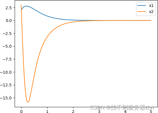
设初值 $x_1(0)=2,x_2(0)=3$，仿真结果如图所示。

simucpp 代码如下

#include <iostream>
#include <cmath>
#include "simucpp.hpp"
using namespace simucpp;
using namespace std;

class Plant: public PackModule {
public:
    Plant(Simulator *sim) {
        intx1 = new UIntegrator(sim, "intx1");
        intx2 = new UIntegrator(sim, "intx2");
        fcnx1 = new UFcnMISO(sim, "fcnx1");
        fcnx2 = new UFcnMISO(sim, "fcnx2");
        in1 = new UGain(sim, "in1");
        sim->connectU(intx1, fcnx1);
        sim->connectU(intx2, fcnx1);
        sim->connectU(in1,   fcnx1);
        sim->connectU(intx1, fcnx2);
        sim->connectU(intx2, fcnx2);
        sim->connectU(in1,   fcnx2);
        sim->connectU(fcnx1, intx1);
        sim->connectU(fcnx2, intx2);
        intx1->Set_InitialValue(2);
        intx2->Set_InitialValue(3);
        fcnx1->Set_Function([](double *u){
            double x1 = u[0], x2 = u[1], u1 = u[2];
            return exp(x1) + x2;
        });
        fcnx2->Set_Function([](double *u){
            double x1 = u[0], x2 = u[1], u1 = u[2];
            return 2*x1*x2*x2 + u1;
        });
    }
private:
    virtual PUnitModule Get_InputPort(uint n=0) const override {
        if (n==0) return in1;
        return nullptr;
    }
    virtual PUnitModule Get_OutputPort(uint n=0) const override {
        if (n==0) return intx1;
        if (n==1) return intx2;
        return nullptr;
    }
    UIntegrator *intx1=nullptr;
    UIntegrator *intx2=nullptr;
    UFcnMISO *fcnx1=nullptr;
    UFcnMISO *fcnx2=nullptr;
    UGain *in1=nullptr;
};

int main() {
    Simulator sim1(5);
    auto *out1 = new UOutput(&sim1, "x1");
    auto *out2 = new UOutput(&sim1, "x2");
    // auto *out3 = new UOutput(&sim1, "alpha");
    auto fcnu = new UFcnMISO(&sim1, "fcnu");
    auto fcnalpha = new UFcnMISO(&sim1, "fcnalpha");
    Plant *plant1 = new Plant(&sim1);
    sim1.connectU(fcnu, plant1, 0);
    sim1.connectU(plant1, 0, fcnu);
    sim1.connectU(plant1, 1, fcnu);
    sim1.connectU(plant1, 0, fcnalpha);
    sim1.connectU(plant1, 1, fcnalpha);
    sim1.connectU(plant1, 0, out1);
    sim1.connectU(plant1, 1, out2);
    sim1.connectU(fcnalpha, fcnu);
    fcnu->Set_Function([](double *u) {
        double x1 = u[0], x2 = u[1], a1=u[2];
        return -2*x1*x2*x2 - (exp(x1)+3)*(exp(x1)+x2)-3*(x2-a1);
    });
    fcnalpha->Set_Function([](double *u) {
        double x1 = u[0], x2 = u[1];
        return -exp(x1)-3*x1;
    });
    sim1.Initialize();
    sim1.Simulate();
    cout << out1->Get_OutValue() << endl;
    cout << out2->Get_OutValue() << endl;
    sim1.Plot();
    return 0;
}