NiagaraFluids代码分析1：力学部分

力学部分

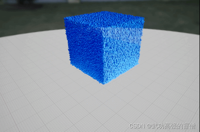
UE5正式版中，Niagara Fluid插件提供了相对完整的流体仿真解决方案，其中模拟部分采用了混合欧拉-拉格朗日视角，使用了PIC/FLIP方法。
本文将就3DLiquidDamBreak粒子系统为出发点，分析其中粒子位置更新的计算过程。
不完整或有错误的地方将在后续学习过程中逐步完善。

1 初始化数据

1.1 Grid 3D Set Resolution

这一部分初始化了Grid的分辨率，即欧拉网格的分辨率。代码如下：

float CellSize = max(WorldGridExtents.z, max(WorldGridExtents.x, WorldGridExtents.y)) / NumCellsMaxAxis;
NumCellsX = floor(WorldGridExtents.x / CellSize);
// step1：取各个方向尺寸的最大值，统一cellsize，再计算每个方向有多少个cell

...
// step2：处理特殊情况，为部分NumCells+1

Out_WorldGridExtents = float3(NumCellsX, NumCellsY, NumCellsZ) * CellSize;
// step3：用上边得到的cellsize和cellnum重新计算在世界空间下模拟的尺寸

1.2 粒子初速度

$$v_{p1}=v_{p0}+((f_p+g)\Delta t)$$

下边对照之前所学的混合欧拉-拉格朗日视角过程，逐层分析

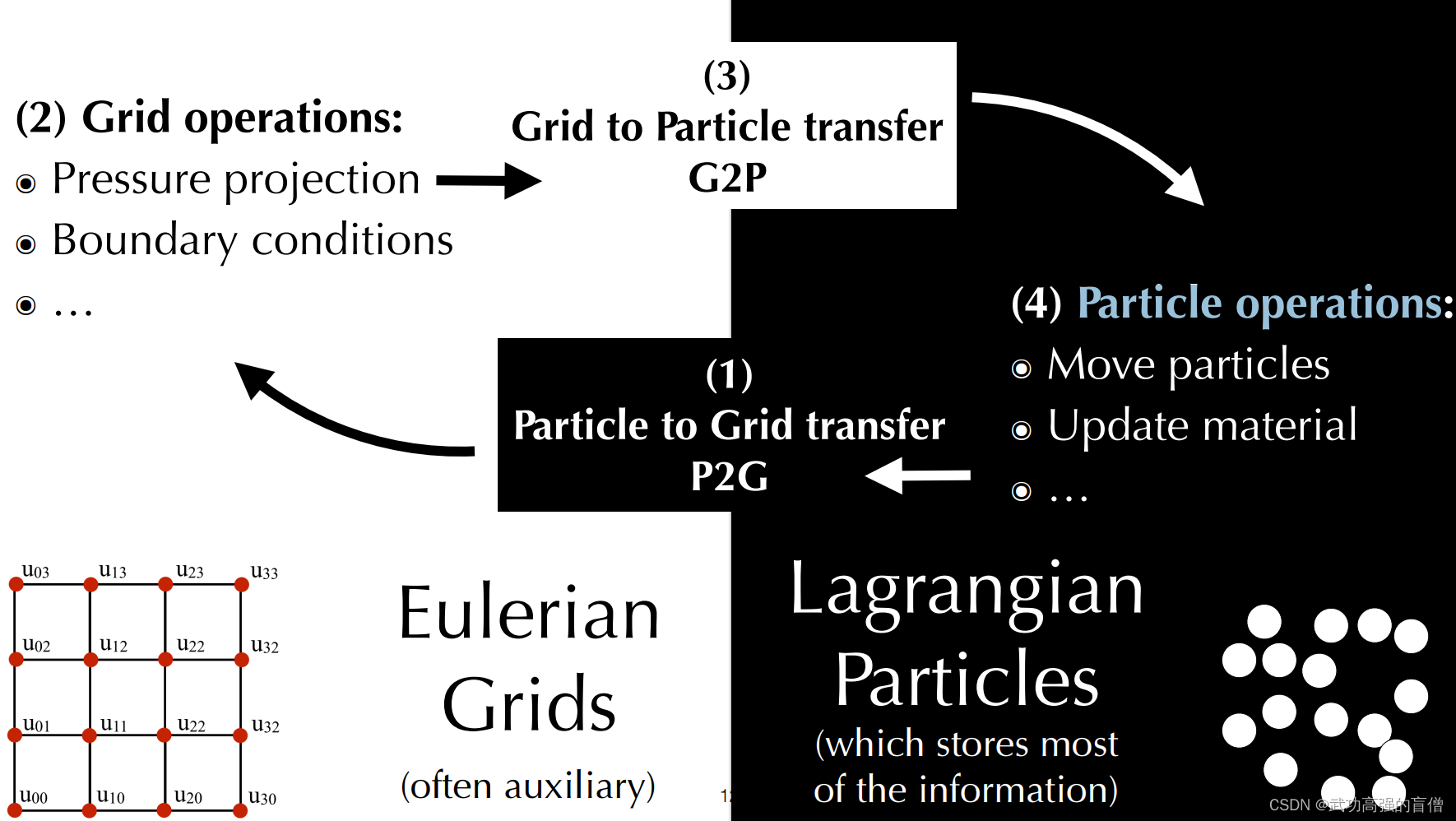
2 P2G Particle to Grid transfer

对应粒子系统中的Rasterize Particles：Grid 3D FLIP Rasterize Particles部分

int IGNORE = 0;

int XIndexInt = floor(Index.x);
int YIndexInt = floor(Index.y);
int ZIndexInt = floor(Index.z); //向下取整到对应的Index，相当于直接存到了粒子所在网格的左上角
for (int x = 0; x <= 1; ++x) {
    for (int y = 0; y <= 1; ++y) {
            for (int z = 0; z <= 1; ++z) {
                const float GridWeightXYZ = 1;//代码中权重均取1
                RasterizationGrid_velocity.InterlockedAddFloatGridValueSafe(XIndexInt+x, YIndexInt+y, ZIndexInt+z, 0, GridWeightXYZ*Velocity.x, IGNORE);
                RasterizationGrid_velocity.InterlockedAddFloatGridValueSafe(XIndexInt+x, YIndexInt+y, ZIndexInt+z, 1, GridWeightXYZ*Velocity.y, IGNORE);
                RasterizationGrid_velocity.InterlockedAddFloatGridValueSafe(XIndexInt+x, YIndexInt+y, ZIndexInt+z, 2, GridWeightXYZ*Velocity.z, IGNORE);
                RasterizationGrid_velocity.InterlockedAddFloatGridValue(XIndexInt+x, YIndexInt+y, ZIndexInt+z, 3, GridWeightXYZ, IGNORE); //分别累加xyz方向的速度到格点上、权重
                BoundaryGrid.SetGridValue(XIndexInt+x, YIndexInt+y, ZIndexInt+z, BoundaryIndex, 3, IGNORE); //记录BoundaryIndex到BoundaryGrid
}}}

参考：Niagara RasterizationGrid3D Data Interface
RasterizationGrid3D可用于迭代源为Particle时并行的累加（InterlockedAddFloatGridValueSafe）

3 Grid operations

3.1 Boundaries conditions

在TransientGrid上存储边界类型和固体速度

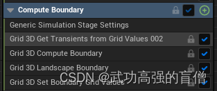
遍历网格TransientGrid，存储当前Index处的边界类型，用于后续计算：

//边界类型
const  int FLUID_CELL = 0; // 0 流体内部
const  int SOLID_CELL = 1; // 1 固体边界
const  int EMPTY_CELL = 2; 

和边界处的固体的速度SolidVelocity

3.2 PIC方法

修正：这里其实可以看作还是P2G的一部分，做的还是在gather速度和处理边界
从RasterizationGrid_velocity中gather速度，若cell处于边界上，则gather所有附近的类型为fluid的cell
代码部分只保留了关键部分

// 从RasterizationGrid_velocity中Gather速度
Grid.GetFloatGridValue(IndexX, IndexY, IndexZ, 0, OutVelocity.x);
Grid.GetFloatGridValue(IndexX, IndexY, IndexZ, 1, OutVelocity.y);
Grid.GetFloatGridValue(IndexX, IndexY, IndexZ, 2, OutVelocity.z);
Grid.GetFloatGridValue(IndexX, IndexY, IndexZ, 3, TmpWeight);
OutVelocity /= TmpWeight;

// if we have a boundary cell, then gather value from closest neighbor cell
// 如果在边界上
[branch]
if (CellType != FLUID_CELL)
{
    // 共采样了3x3x3 = 27个 跳过了不是FLUID_CELL类型的cell
    for (int xx = -ExtrapolationHalfWidth; xx <= ExtrapolationHalfWidth; ++xx)  {
    for (int yy = -ExtrapolationHalfWidth; yy <= ExtrapolationHalfWidth; ++yy)  {        
    for (int zz = -ExtrapolationHalfWidth; zz <= ExtrapolationHalfWidth; ++zz)  { 
        // only extrapolate from fluid cells 
        // don't extrapolate from the boundary of the domain to allow particles to pass through as ballistic when they leave
        if (TmpCellType == FLUID_CELL)
        {
            float Weight = 1./length2(float3(xx,yy,zz));
            // gather邻居
            Grid.GetFloatGridValue(IndexX+xx, IndexY+yy, IndexZ+zz, 0, TmpVelocity.x);
            Grid.GetFloatGridValue(IndexX+xx, IndexY+yy, IndexZ+zz, 1, TmpVelocity.y);
            Grid.GetFloatGridValue(IndexX+xx, IndexY+yy, IndexZ+zz, 2, TmpVelocity.z);
            Grid.GetFloatGridValue(IndexX+xx, IndexY+yy, IndexZ+zz, 3, TmpWeight);

            TmpVelocity /= TmpWeight; // 所在cell的速度
            OutVelocity += TmpVelocity * Weight; // 按照距离平方的倒数作为权重累加
            TotalWeight  += Weight; // 累加权重

        }
    }}}
    OutVelocity /= TotalWeight;
}

gather得到的速度，直接作为SimGrid的$v_i^t$和 $v_i^{t+1}$"（aka. StartVelocity and Velocity）

3.3 Projection

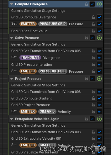
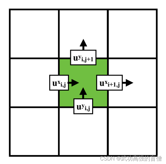
3.3.1 Compute Divergence 计算散度

Div = (Vx_right - Vx_left + Vy_up - Vy_down + Vz_front - Vz_back) / (2. * dx);

对应$\nabla \cdot u$

计算完成后将Div赋值给TemporaryGrid，同时初始化PressureGrid中Pressure值为0

3.3.2 Solve Pressure 解算压力

使用SOR方法迭代50次解算出一个压力场（即Pressure Grid中的值），使散度为0
代码中使用了Red-Black Successive Over-Relaxation (SOR)方法
其中
SOR方法参考：线性方程组的SOR迭代法
Red-Black Ordering方法参考：Red-Black Ordering Lecture 67 Numerical Methods for Engineering
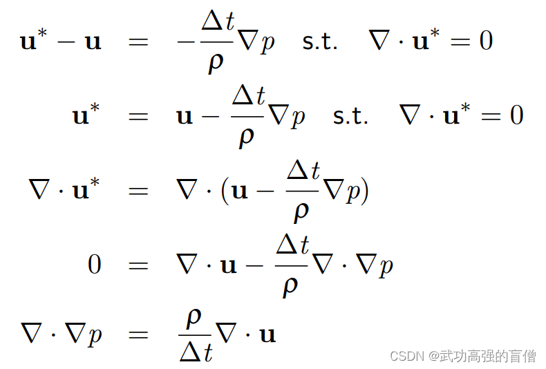
首先，介绍本文中需要求解的矩阵 Ax = b，参考Games201学习笔记3：欧拉视角4. Prjection部分
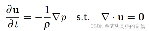
压力对加速度的贡献

对方程展开，$\frac{\partial u}{\partial t}$替换为下一时刻速度-当前速度，移项，左右同时求散度 $\nabla \cdot$由于下一时刻散度为0，所以 $\nabla \cdot u^{\ast }=0$项消去，化简的到最后结果

左边一项采用中心差分法近似拉普拉斯（三维空间下为上下左右前后的邻居，其中4$p_{i,j}$中的4替换为周围cell类型为fluid或empty的个数（FluidCellCount），代码如下

float Scale = dx / dt;
int CellType_right = round(B_right);
if (CellType_right == SOLID_CELL)
{
    FluidCellCount--;//从6递减
    BoundaryAdd += Scale * (Velocity.x - SV_x_right);//固体边界的相对速度提供的压力
    P_right = 0;//若边界不是fluid则压力为0
}
else if (CellType_right == EMPTY_CELL)
{
   P_right = 0;
}

右边式子中的散度已知，ρ取了1，故得到以下等式
$$\frac{1}{\Delta x^2}(-FluidCellCount\times P_{center}+P_{right}+P_{left}+P_{up}+P_{down}+P_{front}+P_{back}+P_{Boundary})=\frac{\nabla \cdot u}{\Delta t}$$

化简
$$P_{center}=(P_{center}+P_{right}+P_{left}+P_{up}+P_{down}+P_{front}+P_{back}+P_{Boundary}-\frac{\Delta x^2\times \nabla \cdot u}{\Delta t})/FluidCellCount$$

对应线性方程Ax=b，其中右边的量均能在一次迭代中求出，作为b，单位向量I作为A，$P_{center}$作为x
解方程使用了Red-Black Successive Over-Relaxation (SOR)方法
先来谈Red-Black：

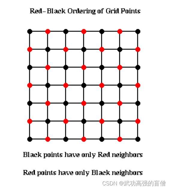
每次迭代，只计算Grid中标记为黑色的部分，下一次迭代，计算红色的部分，交替进行。判断当前格点颜色的代码如下，CellParity的值为0或1表示红黑

int SliceParity = (IndexZ + IterationIndex) % 2;
int RowParity = (IndexY + SliceParity+1) % 2;
int CellParity = (IndexX + RowParity ) % 2;

// will do red-black SOR
// add 1 since we want to expose a 0-1 parameter
Weight = CellParity * min(1.93, Relaxation + 1);

再来谈SOR：Successive Over Relaxation（逐次超松弛），是Gauss-Seidel迭代法的加速，引入了ω加速迭代。具体推导参考上边链接，这里直接把结果拿来了

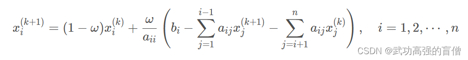
前边提到A为单位矩阵，故只有aii=1，其他为0，化简如下，ω对应上述的weight，经过红黑优化后的权重，具体使用时Relaxation = 0.95，故ω=1.93或0

$$x_i^{k+1}=(1-\omega )x_i^k+\omega b_i$$

$$P_{center}=(P_{center}+P_{right}+P_{left}+P_{up}+P_{down}+P_{front}+P_{back}+P_{Boundary}-\frac{\Delta x^2\times \nabla \cdot u}{\Delta t})/FluidCellCount$$

综上，对应代码

if (FluidCellCount > 0) 
{
    float JacobiPressure = (P_right + P_left + P_up + P_down + P_front + P_back -  dx * dx * Divergence / dt + BoundaryAdd) / FluidCellCount;
    Pressure = (1.f - Weight) * P_center + Weight * JacobiPressure;
}

共迭代50次后，得到一个散度近似为0的压力场，记录在Pressure Grid中

3.3.4 Project Pressure

将p带入公式求速度，同时处理边界问题

step1：求梯度$\nabla p$，由邻居的pressure近似梯度Gradient

Grad = float3(S_right - S_left, S_up - S_down, S_front - S_back) / (2.0 * dx);

step2：求加速度

step3：处理边界（以左右边界为例，后边处理上下，前后同理）

//只考虑一边是边界，而非左右都是边界的极端情况
if (CellType_left == SOLID_CELL)
{
    VelocityOut.x = SV_x_left; //左边为边界，则从边界中读取速度并赋值
}
else if (CellType_right == SOLID_CELL)
{
    VelocityOut.x = SV_x_right; 
}
else
{
    VelocityOut.x = Velocity.x; //上下都不是边界，则正常赋值
}

得到的速度赋给SimGrid保存

3.3.5 Extrapolate Velocities Again

在SimGrid上处理cell类型为边界的值，相当于模糊了边界速度值，同3.2

3.4 小结

至此，新的速度场已经计算得到，存储在SimGrid中，下边将使用PIC/FLIP方法，更新速度到粒子上。旧的速度场在第一次Extrapolate Velocities时，也记录到了SimGrid，使用了不同的下标（AttributeIndex）

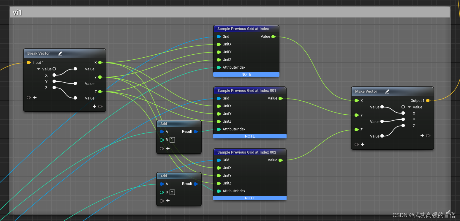
4 G2P Grid to Particle transfer

这里开始Simulation Stage的迭代源为particle，之前的迭代源为Grid
UE这里使用的方法为将particle的坐标进行2次矩阵乘法（SimulationToWorld，WorldToUnit），输出位置为UnitPos，一般是0-1的float，超出范围的不再更新速度，只按照当前速度更新位置

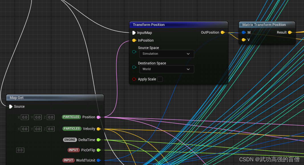
然后用unitpos在SimGrid网格中插值采样得到速度，插值的代码没有看到，盲猜是三维空间下的线性插值。

5 Particle operations

5.1 Move particle

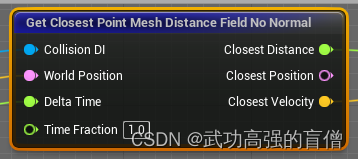
边界的处理：
若粒子处于固体边界中，速度取0，位置不变
若粒子处于空cell中，速度不变，位置按照当前粒子速度乘以dt更新

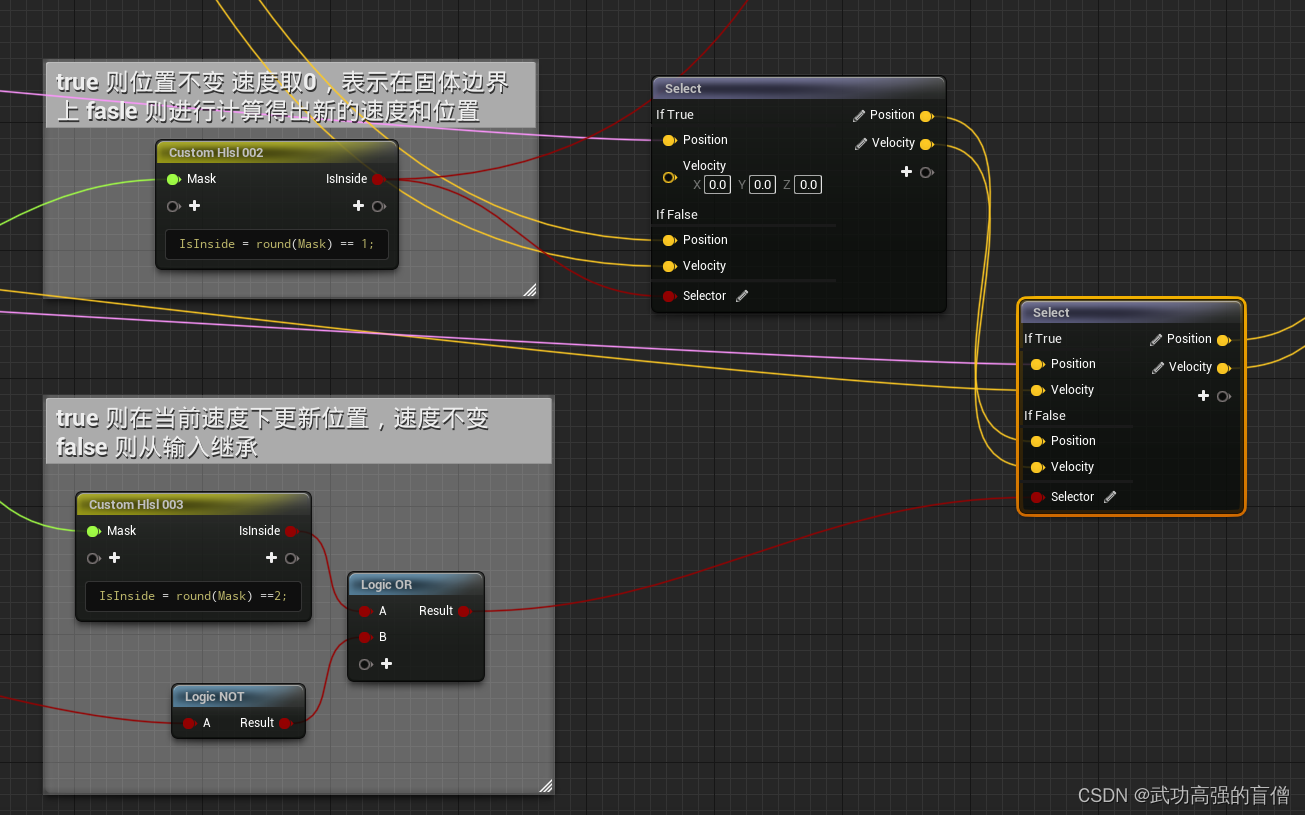
若不在以上边界，速度的更新则按照PIC/FLIP方法混合更新。
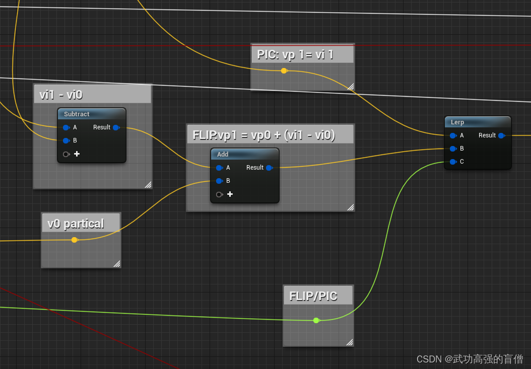
回顾这2种方法：

1. PIC：$v_p^{t+1}=v_i^{t+1}$直接从网格中采样得到并更新
2. FLIP：$v_p^{t+1}=v_p^t+gather(v_i^{t+1}-v_i^t)$ 从网格中采样速度的增量，累加到原来的速度上

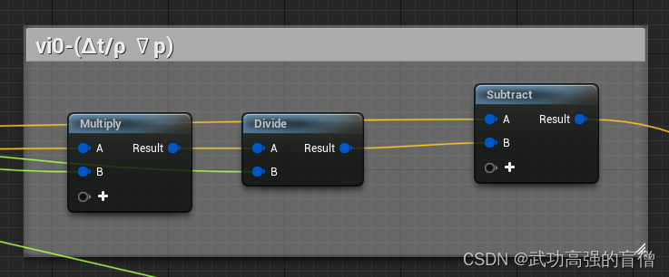
蓝图中如下表示

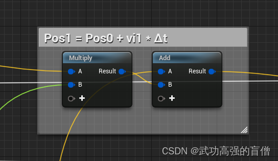
位置的更新略有不同，完全使用了PIC方法，即直接使用网格中采样得到新的速度场更新粒子位置

6 总结

至此，力学部分的计算过程总结完成，遗留了渲染得到水的部分，将在下一篇中更新