


🧑 博主简介:曾任某智慧城市类企业
算法总监,目前在美国市场的物流公司从事高级算法工程师一职,深耕人工智能领域,精通python数据挖掘、可视化、机器学习等,发表过AI相关的专利并多次在AI类比赛中获奖。CSDN人工智能领域的优质创作者,提供AI相关的技术咨询、项目开发和个性化解决方案等服务,如有需要请站内私信或者联系任意文章底部的的VX名片(ID:xf982831907)
💬 博主粉丝群介绍:① 群内初中生、高中生、本科生、研究生、博士生遍布,可互相学习,交流困惑。② 热榜top10的常客也在群里,也有数不清的万粉大佬,可以交流写作技巧,上榜经验,涨粉秘籍。③ 群内也有职场精英,大厂大佬,可交流技术、面试、找工作的经验。④ 进群免费赠送写作秘籍一份,助你由写作小白晋升为创作大佬。⑤ 进群赠送CSDN评论防封脚本,送真活跃粉丝,助你提升文章热度。有兴趣的加文末联系方式,备注自己的CSDN昵称,拉你进群,互相学习共同进步。

【数据可视化-51】基于时间序列的电力负荷数据可视化探索
一、引言
随着全球气候变化和能源需求的不断增长,理解和预测电力负荷已成为能源管理和规划的关键。电力负荷受到多种因素的影响,其中天气条件(如温度、湿度、风速和辐射强度)是最重要的因素之一。通过分析天气参数与电力负荷之间的关系,我们可以更好地预测电力需求,优化能源分配,并制定有效的能源管理策略。本文将使用 matplotlib 库对艾哈迈达巴德地区的天气和电力负荷数据集进行可视化分析,探索不同天气条件对电力负荷的影响。
二、数据集介绍
本次分析所使用的数据集结合了艾哈迈达巴德地区每小时的电力负荷变化和天气参数。数据集包含以下 10 个特征:
- Year:年份
- Month:月份
- Day:日期
- Hour:小时
- irradiance:辐射强度
- temperature:温度
- dewpoint:露点温度
- specific humidity:比湿度
- wind speed:风速
- Electric Load (MW):电力负荷(兆瓦)
数据来源于 NASA 开源网站的天气参数和艾哈迈达巴德变电站的电力负荷记录。
2.1 导入数据与预处理
在开始可视化分析之前,我们需要先导入数据并进行必要的预处理。
import numpy as np
import pandas as pd
import matplotlib.pyplot as plt
from wordcloud import WordCloud
from collections import Counter
import string

# 导入数据
df = pd.read_csv('weather_electric_load_dataset.csv')


# 查看数据基本信息
print("数据大小:", df.shape)
print("\n数据基本信息:")
print(df.info())
print("\n数据描述性统计:")
print(df.describe())

# 统计缺失值
print("\n缺失值统计:")
print(df.isnull().sum())

# 统计重复值
print("\n重复值数量:", df.duplicated().sum())
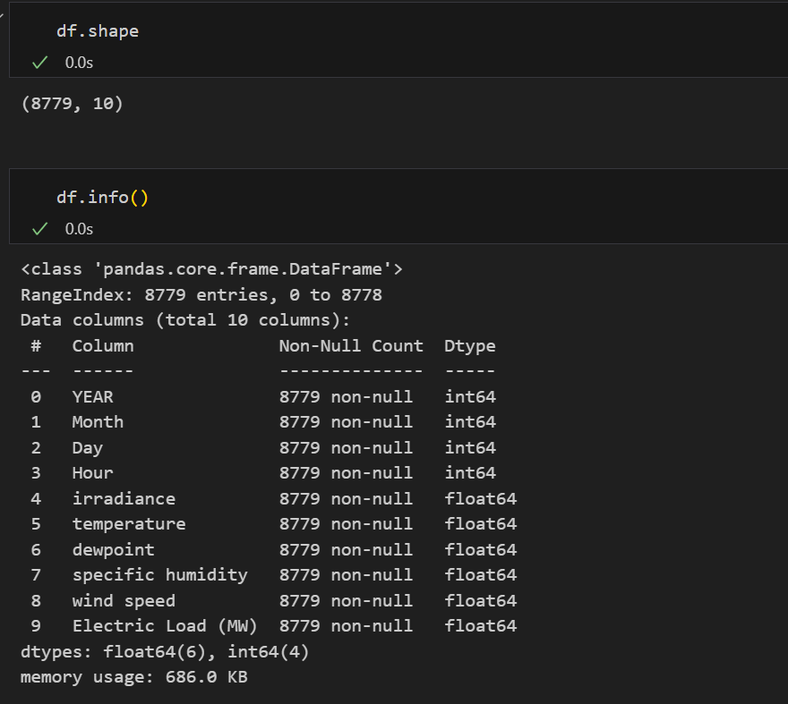
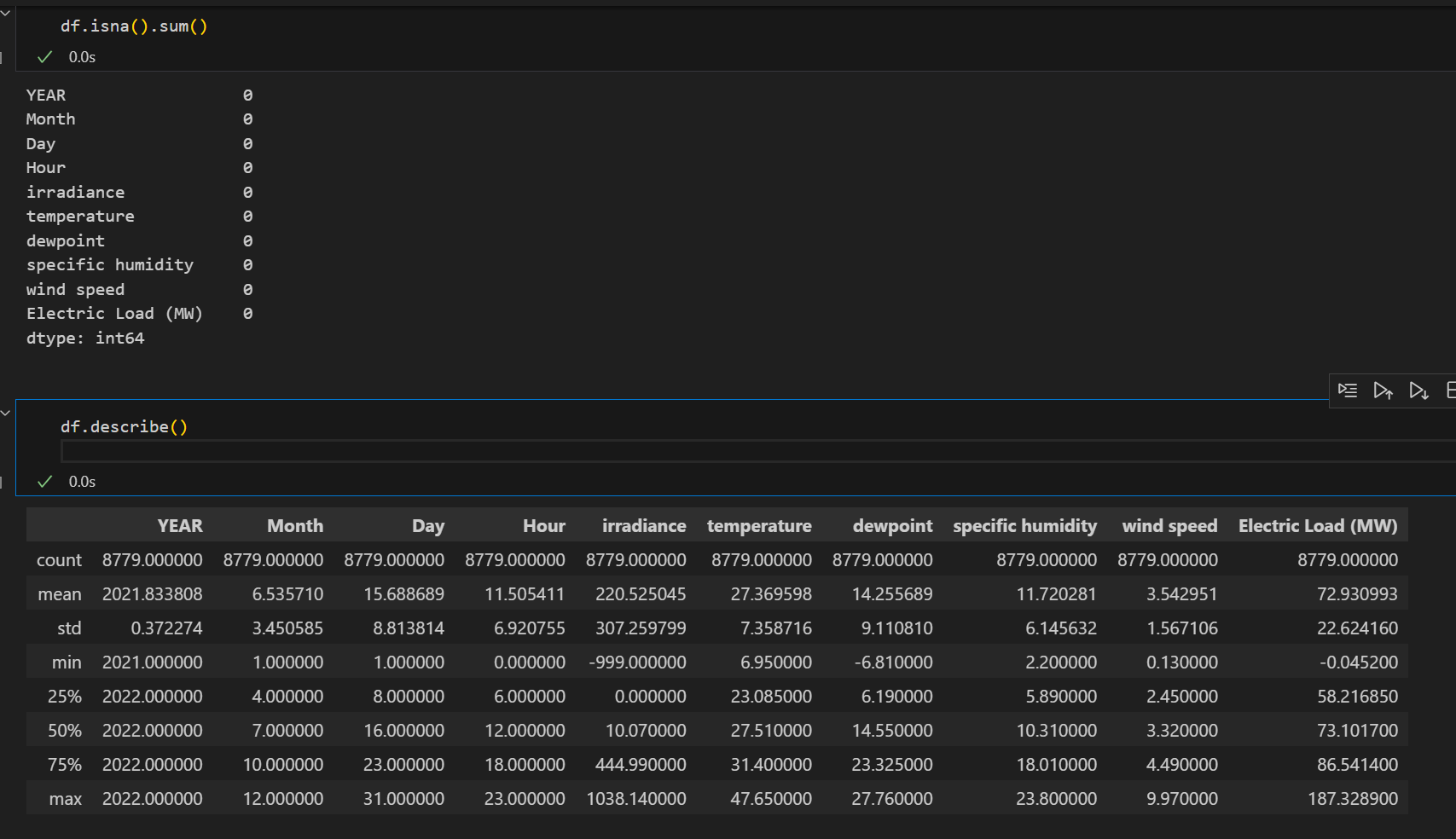
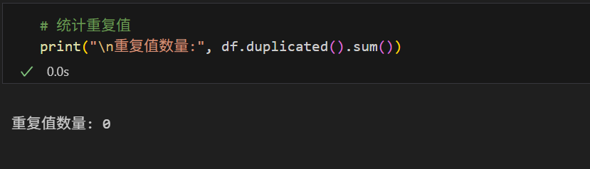
从上面的分析可以发现:
- 数据中包含10个字段,8779条数据,无缺失值和重复值;
- 年月日小时等字段都是int类型,其它特征都为float类型,后续需要将年月日小时转换城日期格式;
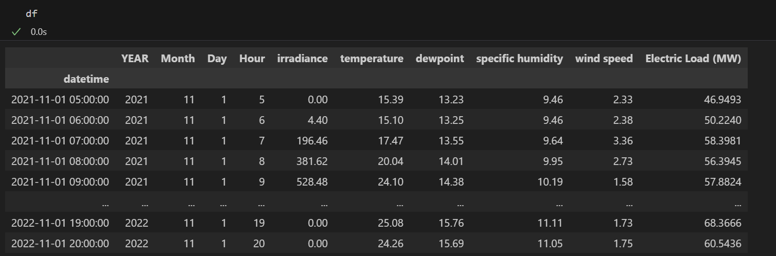
# 转换日期时间格式
df['datetime'] = pd.to_datetime(df[['YEAR', 'Month', 'Day', 'Hour']].assign(Hour=df['Hour'].apply(lambda x: f"{x:02d}")))
df.set_index('datetime', inplace=True)
三、单变量分析
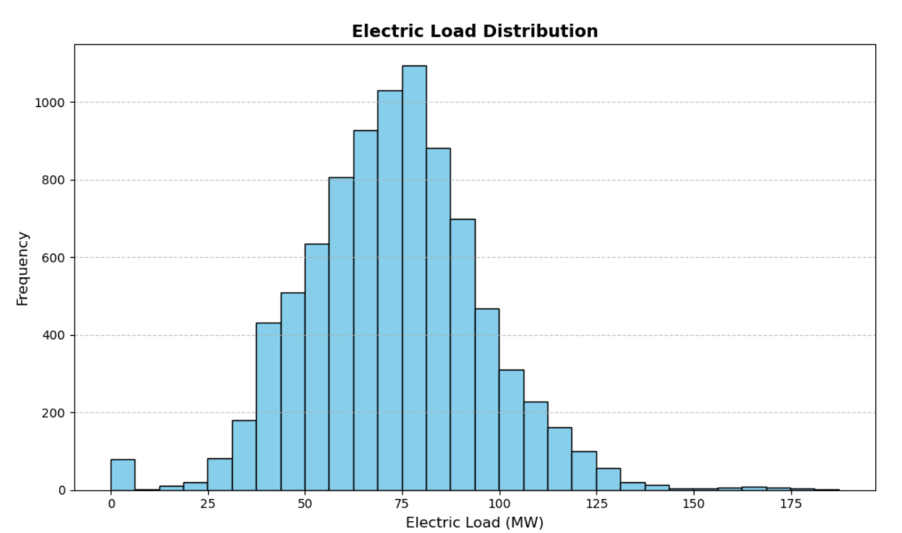
3.1 电力负荷分布
首先,我们分析电力负荷的分布情况,了解其变化范围和集中趋势。
plt.figure(figsize=(10, 6))
plt.hist(df['Electric Load (MW)'].dropna(), bins=30, color='skyblue', edgecolor='black')
plt.title('Electric Load Distribution', fontsize=14, fontweight='bold')
plt.xlabel('Electric Load (MW)', fontsize=12)
plt.ylabel('Frequency', fontsize=12)
plt.grid(axis='y', linestyle='--', alpha=0.7)
plt.tight_layout()
plt.show()
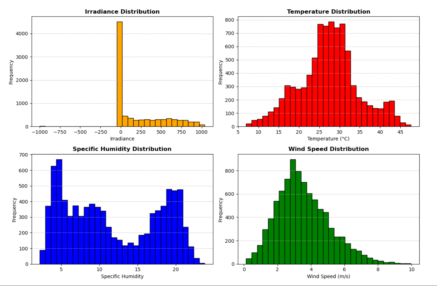
3.2 天气参数分布
接下来,我们分析各个天气参数的分布情况,包括辐射强度、温度、湿度和风速。
fig, axes = plt.subplots(2, 2, figsize=(12, 8))
axes = axes.flatten()

# 辐射强度分布
axes[0].hist(df['irradiance'].dropna(), bins=30, color='orange', edgecolor='black')
axes[0].set_title('Irradiance Distribution', fontsize=12, fontweight='bold')
axes[0].set_xlabel('Irradiance', fontsize=10)
axes[0].set_ylabel('Frequency', fontsize=10)
axes[0].grid(axis='y', linestyle='--', alpha=0.7)

# 温度分布
axes[1].hist(df['temperature'].dropna(), bins=30, color='red', edgecolor='black')
axes[1].set_title('Temperature Distribution', fontsize=12, fontweight='bold')
axes[1].set_xlabel('Temperature (°C)', fontsize=10)
axes[1].set_ylabel('Frequency', fontsize=10)
axes[1].grid(axis='y', linestyle='--', alpha=0.7)

# 湿度分布
axes[2].hist(df['specific humidity'].dropna(), bins=30, color='blue', edgecolor='black')
axes[2].set_title('Specific Humidity Distribution', fontsize=12, fontweight='bold')
axes[2].set_xlabel('Specific Humidity', fontsize=10)
axes[2].set_ylabel('Frequency', fontsize=10)
axes[2].grid(axis='y', linestyle='--', alpha=0.7)

# 风速分布
axes[3].hist(df['wind speed'].dropna(), bins=30, color='green', edgecolor='black')
axes[3].set_title('Wind Speed Distribution', fontsize=12, fontweight='bold')
axes[3].set_xlabel('Wind Speed (m/s)', fontsize=10)
axes[3].set_ylabel('Frequency', fontsize=10)
axes[3].grid(axis='y', linestyle='--', alpha=0.7)

plt.tight_layout()
plt.show()
四、时间序列分析
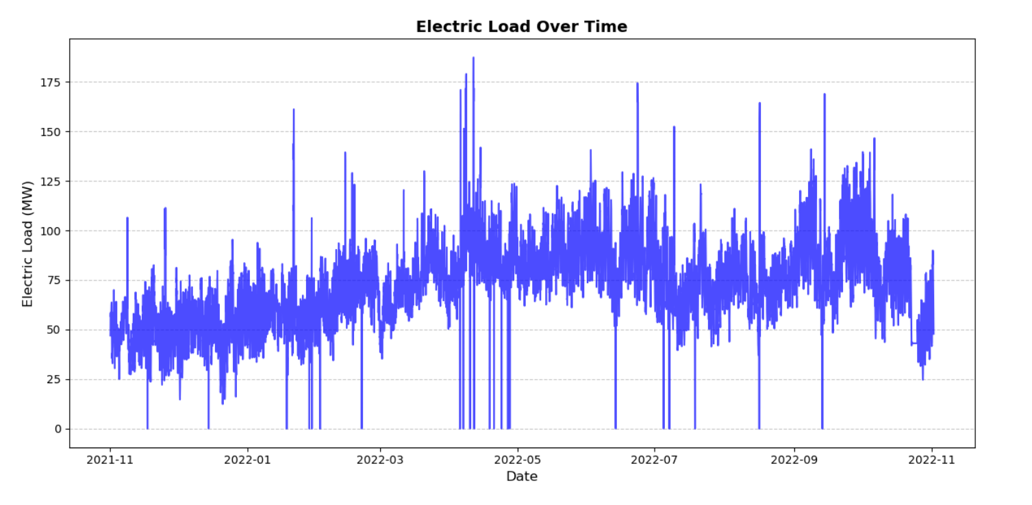
4.1 电力负荷随时间变化
分析电力负荷随时间的变化趋势,了解其日、月、年的变化规律。
plt.figure(figsize=(12, 6))
plt.plot(df.index, df['Electric Load (MW)'], color='blue', alpha=0.7)
plt.title('Electric Load Over Time', fontsize=14, fontweight='bold')
plt.xlabel('Date', fontsize=12)
plt.ylabel('Electric Load (MW)', fontsize=12)
plt.grid(axis='y', linestyle='--', alpha=0.7)
plt.tight_layout()
plt.show()
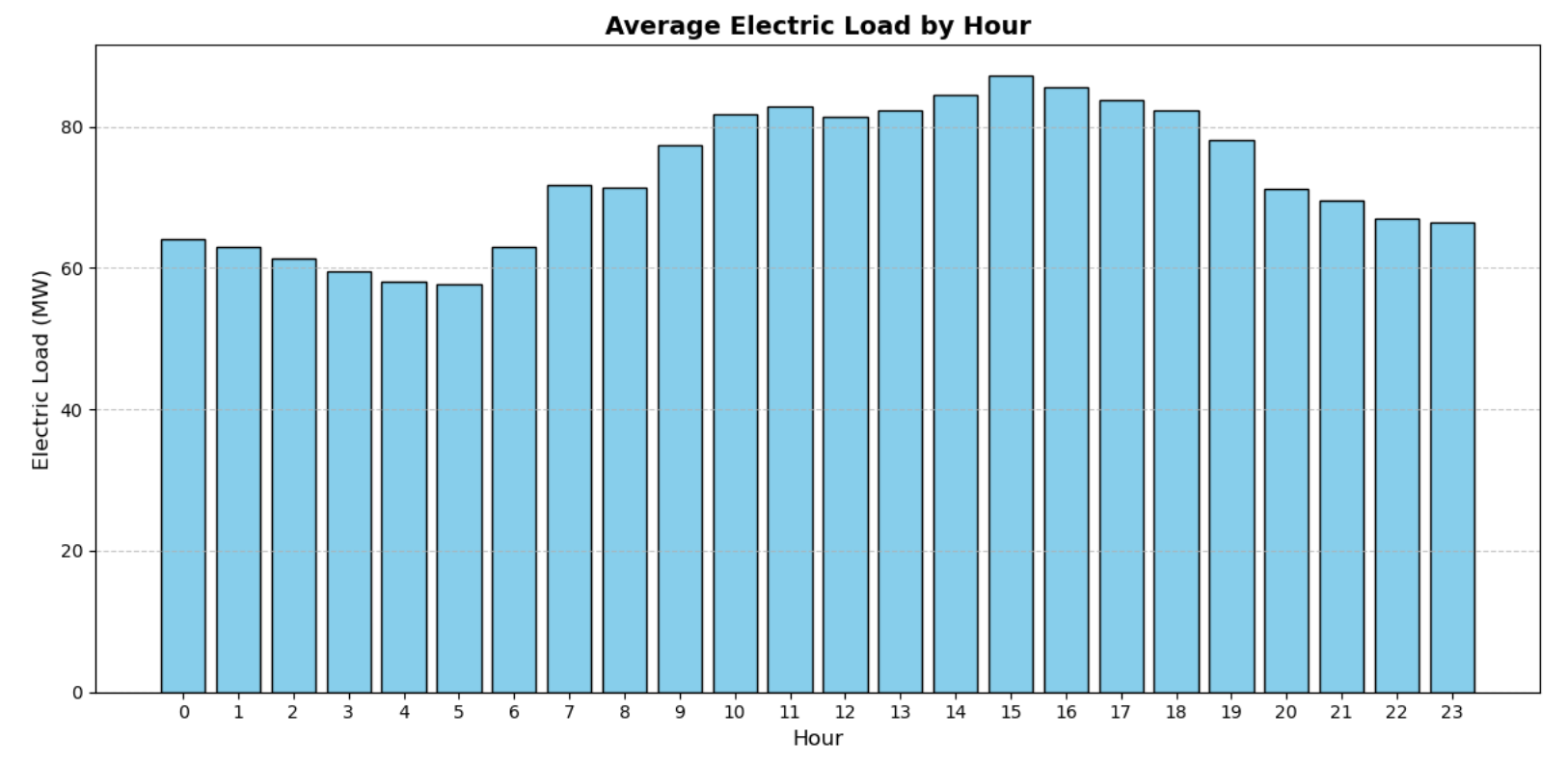
4.2 各小时电力负荷平均值
分析不同时间段的电力负荷变化,找出负荷高峰和低谷。
hourly_load = df.groupby(df.index.hour)['Electric Load (MW)'].mean()

plt.figure(figsize=(12, 6))
plt.bar(hourly_load.index, hourly_load.values, color='skyblue', edgecolor='black')
plt.title('Average Electric Load by Hour', fontsize=14, fontweight='bold')
plt.xlabel('Hour', fontsize=12)
plt.ylabel('Electric Load (MW)', fontsize=12)
plt.xticks(hourly_load.index)
plt.grid(axis='y', linestyle='--', alpha=0.7)
plt.tight_layout()
plt.show()
五、多变量分析
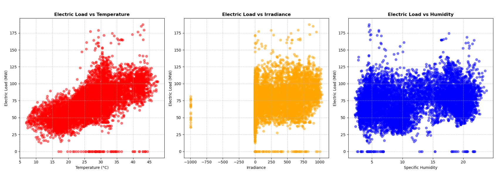
5.1 电力负荷与天气参数的关系
分析温度、辐射强度、湿度和风速对电力负荷的影响。
fig, axes = plt.subplots(1, 3, figsize=(18, 6))
axes = axes.flatten()

# 电力负荷与温度
axes[0].scatter(df['temperature'], df['Electric Load (MW)'], alpha=0.5, color='red')
axes[0].set_title('Electric Load vs Temperature', fontsize=12, fontweight='bold')
axes[0].set_xlabel('Temperature (°C)', fontsize=10)
axes[0].set_ylabel('Electric Load (MW)', fontsize=10)
axes[0].grid(axis='both', linestyle='--', alpha=0.7)

# 电力负荷与辐射强度
axes[1].scatter(df['irradiance'], df['Electric Load (MW)'], alpha=0.5, color='orange')
axes[1].set_title('Electric Load vs Irradiance', fontsize=12, fontweight='bold')
axes[1].set_xlabel('Irradiance', fontsize=10)
axes[1].set_ylabel('Electric Load (MW)', fontsize=10)
axes[1].grid(axis='both', linestyle='--', alpha=0.7)

# 电力负荷与湿度
axes[2].scatter(df['specific humidity'], df['Electric Load (MW)'], alpha=0.5, color='blue')
axes[2].set_title('Electric Load vs Humidity', fontsize=12, fontweight='bold')
axes[2].set_xlabel('Specific Humidity', fontsize=10)
axes[2].set_ylabel('Electric Load (MW)', fontsize=10)
axes[2].grid(axis='both', linestyle='--', alpha=0.7)

plt.tight_layout()
plt.show()
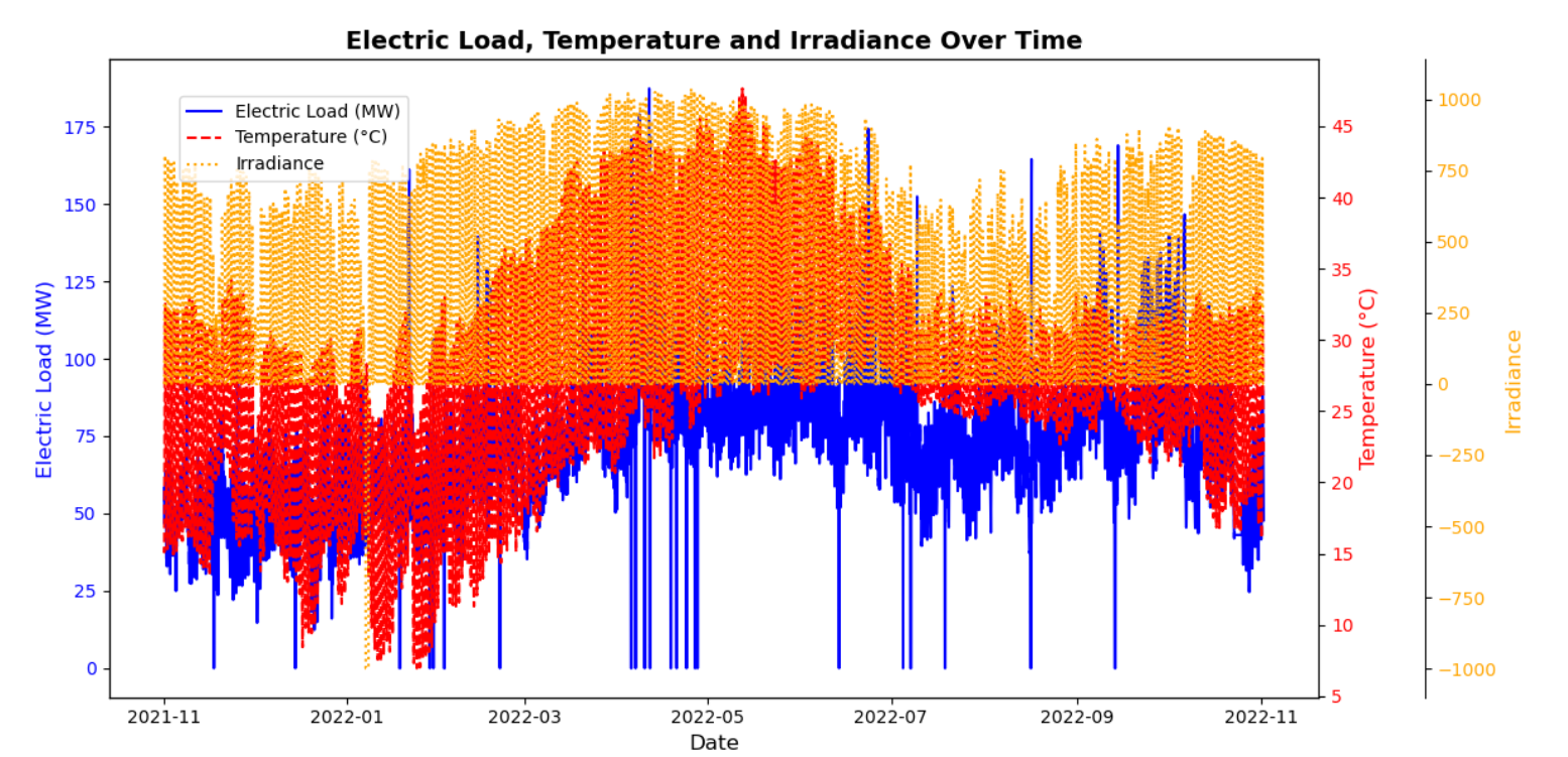
5.2 组合图表:电力负荷、温度和辐射强度随时间变化
将电力负荷、温度和辐射强度的变化趋势绘制在同一图表中,直观展示它们之间的关系。
fig, ax1 = plt.subplots(figsize=(12, 6))

# 电力负荷
ax1.plot(df.index, df['Electric Load (MW)'], label='Electric Load (MW)', color='blue')
ax1.set_xlabel('Date', fontsize=12)
ax1.set_ylabel('Electric Load (MW)', fontsize=12, color='blue')
ax1.tick_params(axis='y', labelcolor='blue')

# 温度
ax2 = ax1.twinx()
ax2.plot(df.index, df['temperature'], label='Temperature (°C)', color='red', linestyle='--')
ax2.set_ylabel('Temperature (°C)', fontsize=12, color='red')
ax2.tick_params(axis='y', labelcolor='red')

# 辐射强度
ax3 = ax1.twinx()
ax3.spines['right'].set_position(('outward', 60))
ax3.plot(df.index, df['irradiance'], label='Irradiance', color='orange', linestyle=':')
ax3.set_ylabel('Irradiance', fontsize=12, color='orange')
ax3.tick_params(axis='y', labelcolor='orange')

fig.legend(loc='upper left', bbox_to_anchor=(0.1, 0.9))
plt.title('Electric Load, Temperature and Irradiance Over Time', fontsize=14, fontweight='bold')
plt.tight_layout()
plt.show()
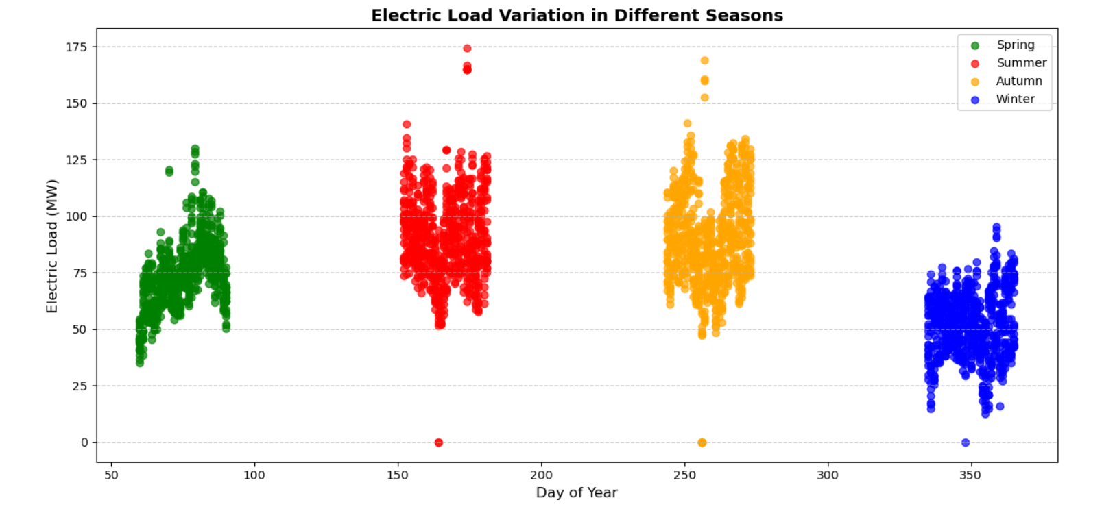
六、季节性分析
6.1 电力负荷的季节性变化
分析不同季节的电力负荷变化,了解季节对电力需求的影响。
seasons = [(3, 'Spring'), (6, 'Summer'), (9, 'Autumn'), (12, 'Winter')]
colors = ['green', 'red', 'orange', 'blue']

fig, ax = plt.subplots(figsize=(12, 6))
for month, season in seasons:
    season_data = df[df.index.month == month]
    ax.scatter(season_data.index.dayofyear, season_data['Electric Load (MW)'], label=season, alpha=0.7, color=colors.pop(0))

ax.set_title('Electric Load Variation in Different Seasons', fontsize=14, fontweight='bold')
ax.set_xlabel('Day of Year', fontsize=12)
ax.set_ylabel('Electric Load (MW)', fontsize=12)
ax.legend()
ax.grid(axis='y', linestyle='--', alpha=0.7)
plt.tight_layout()
plt.show()
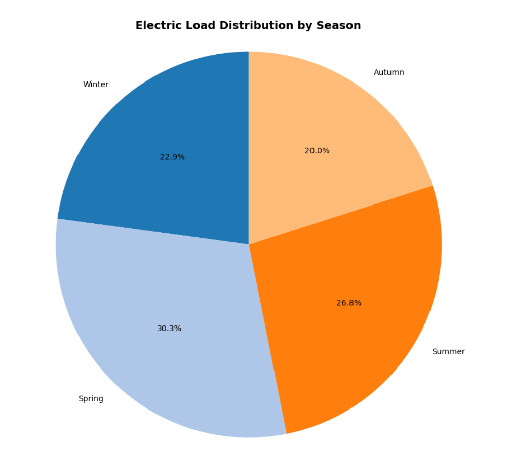
6.2 季节性电力负荷分布
使用饼图展示不同季节的电力负荷分布情况。
seasonal_load = df.groupby(df.index.quarter)['Electric Load (MW)'].mean()
season_labels = ['Winter', 'Spring', 'Summer', 'Autumn']

plt.figure(figsize=(8, 8))
plt.pie(seasonal_load, labels=season_labels, autopct='%1.1f%%', colors=plt.cm.tab20.colors, startangle=90)
plt.title('Electric Load Distribution by Season', fontsize=14, fontweight='bold')
plt.axis('equal')
plt.tight_layout()
plt.show()
七、相关性分析
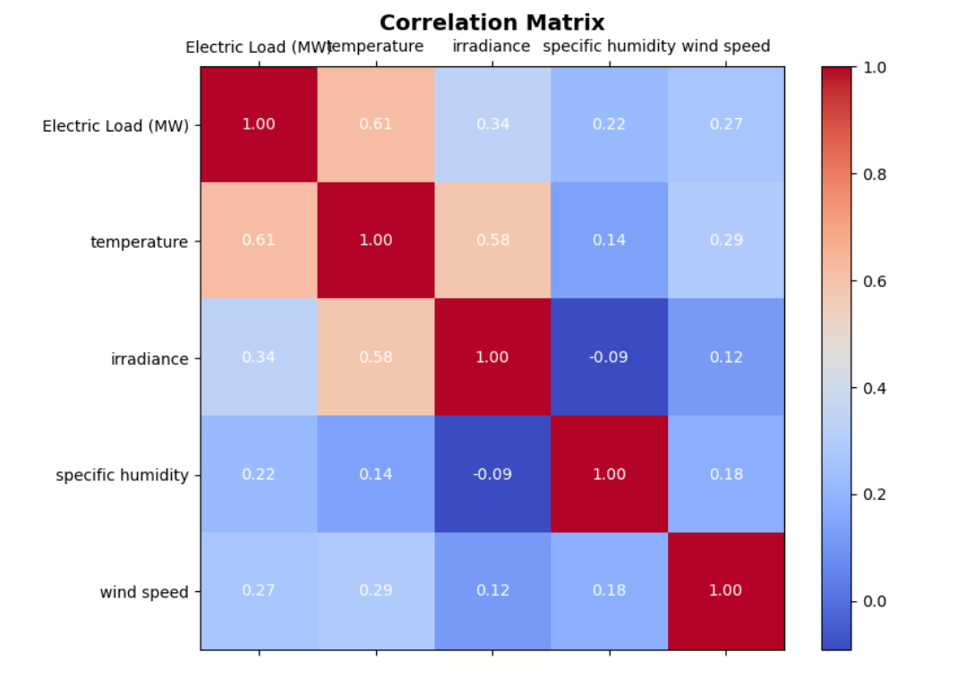
7.1 天气参数与电力负荷的相关性
分析天气参数与电力负荷之间的相关性,找出影响电力负荷的主要因素。
correlation_matrix = df[['Electric Load (MW)', 'temperature', 'irradiance', 'specific humidity', 'wind speed']].corr()

fig, ax = plt.subplots(figsize=(8, 6))
cax = ax.matshow(correlation_matrix, cmap='coolwarm')
fig.colorbar(cax)

for i in range(correlation_matrix.shape[0]):
    for j in range(correlation_matrix.shape[1]):
        ax.text(j, i, f"{correlation_matrix.iloc[i, j]:.2f}", ha='center', va='center', color='white')

ax.set_xticks(range(len(correlation_matrix.columns)))
ax.set_yticks(range(len(correlation_matrix.columns)))
ax.set_xticklabels(correlation_matrix.columns)
ax.set_yticklabels(correlation_matrix.columns)
ax.set_title('Correlation Matrix', fontsize=14, fontweight='bold')
plt.tight_layout()
plt.show()
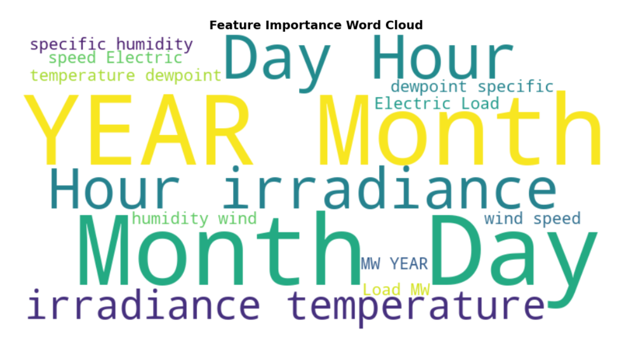
八、特征重要性词云
8.1 天气参数重要性词云
使用词云图展示天气参数对电力负荷的重要性。
text = ' '.join(df.columns.tolist() * 100)  # 使用特征名称创建文本

wordcloud = WordCloud(width=800, height=400, background_color='white').generate(text)

plt.figure(figsize=(10, 6))
plt.imshow(wordcloud, interpolation='bilinear')
plt.title('Feature Importance Word Cloud', fontsize=14, fontweight='bold')
plt.axis('off')
plt.tight_layout()
plt.show()
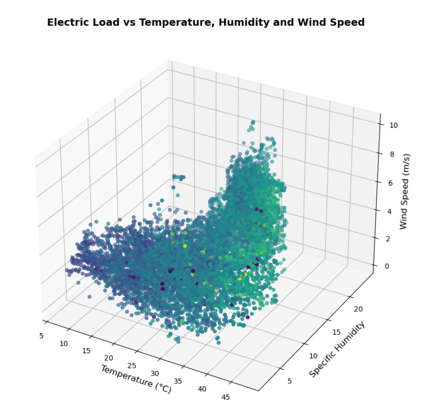
九、多维度组合分析
9.1 3D 散点图:电力负荷与温度、湿度、风速的关系
在一个 3D 图中展示电力负荷与温度、湿度、风速之间的关系。
from mpl_toolkits.mplot3d import Axes3D

fig = plt.figure(figsize=(12, 8))
ax = fig.add_subplot(111, projection='3d')

ax.scatter(df['temperature'], df['specific humidity'], df['wind speed'], c=df['Electric Load (MW)'], cmap='viridis', marker='o')

ax.set_xlabel('Temperature (°C)', fontsize=12)
ax.set_ylabel('Specific Humidity', fontsize=12)
ax.set_zlabel('Wind Speed (m/s)', fontsize=12)
ax.set_title('Electric Load vs Temperature, Humidity and Wind Speed', fontsize=14, fontweight='bold')

plt.tight_layout()
plt.show()
十、总结
通过对艾哈迈达巴德地区的天气和电力负荷数据集的可视化分析,我们可以得出以下结论:
-
电力负荷分布:电力负荷呈现出明显的日变化和季节变化规律,通常在下午和傍晚达到高峰。
-
天气参数影响:温度、辐射强度和湿度对电力负荷有显著影响。温度升高通常会导致电力负荷增加,尤其是在夏季。
-
季节性变化:不同季节的电力负荷存在显著差异,夏季通常是电力负荷的高峰期。
-
相关性分析:温度与电力负荷之间的相关性最高,其次是辐射强度和湿度。
-
多维度关系:通过 3D 散点图可以更直观地看到温度、湿度和风速对电力负荷的综合影响。
这些发现对于电力公司进行电力负荷预测、优化电力资源分配和制定应对策略具有重要意义。通过进一步的机器学习模型开发,可以利用这些天气参数来构建更准确的电力负荷预测模型,从而提高能源利用效率和电网稳定性。
以上代码和分析可以作为数据可视化博客的基础,帮助读者理解天气条件对电力负荷的影响,并为能源管理和规划提供数据支持。
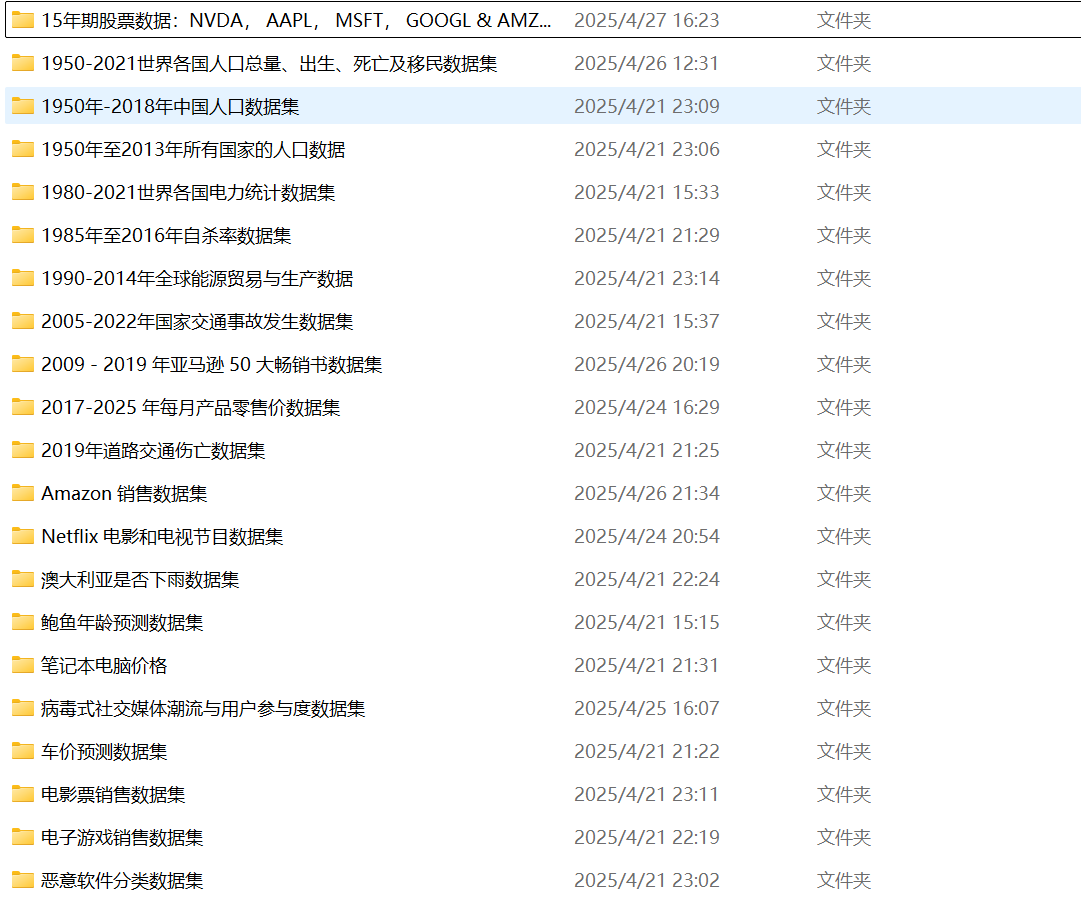
注: 博主目前收集了6900+份相关数据集,有想要的可以领取部分数据:


 2万+
2万+

 被折叠的 条评论
为什么被折叠?
被折叠的 条评论
为什么被折叠?
 到【灌水乐园】发言


