Open3d入门

点云兔子

已于 2023-02-22 14:43:02 修改

阅读量948

点赞数

分类专栏： Open3d点云处理文章标签： python open3d 三维点云 pca 体素

于 2023-02-21 17:06:07 首次发布

本文链接：https://blog.csdn.net/qq_40301351/article/details/129139935

版权

Open3d点云处理专栏收录该内容

1 篇文章 0 订阅

订阅专栏

点云数据

常用数据下载（免积分）

1 主成分分析

1.1 Method

对点云进行主成分分析（PCA）的方法主要有三个步骤：

(1)通过中心进行归一化：

$\tilde{X}=[\tilde{x_1},\tilde{x_2},...,\tilde{x_m}],\tilde{x_i}=x_i-\bar{x},i=1,...,m$

(2)计算SVD或相关性：

$H=\tilde{X}\tilde{X}^T=U_r\Sigma^2U_r^T$

$H=\frac{1}{n}XX^T$

(3)主向量是Ur的列向量。(X的特征向量=H的特征向量)。

1.2 Results

代码展示

def PCA(data, correlation=False, sort=True):
    """
    Apply PCA to point cloud
    Args:
        data: point cloud, matrix of Nx3
        correlation: use np.cov if False, otherwise np.corrcoef if True. default: False
        sort: whether sort according to eigenvalues. default: True.
    Returns:
        eigenvalues
        eigenvectors
    """
    # 1. compute the covariance matrix
    if correlation:
        # each row represents a variable, and each column a single observation of all those variables.
        cov_mat = np.corrcoef(data.T)
    else:
        cov_mat = np.cov(data.T)

    # 2. apply svd to the covariance matrix
    eigenvalues, eigenvectors = np.linalg.eig(cov_mat)

    if sort:
        sort = eigenvalues.argsort()[::-1]
        eigenvalues = eigenvalues[sort]
        eigenvectors = eigenvectors[:, sort]

    return eigenvalues, eigenvectors

结果展示

主方向

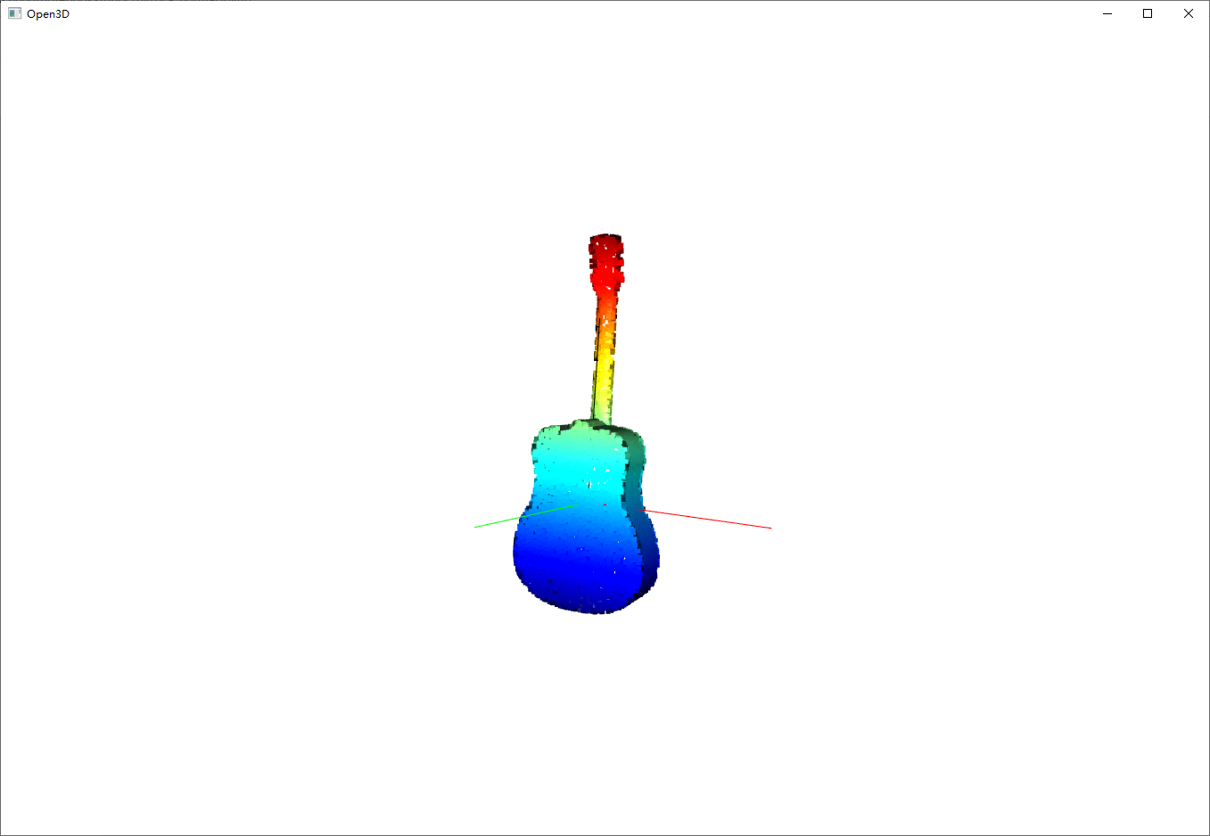
投影

2 表面法线估计

2.1 Method

三维点云的表面法线估计方法主要有三个步骤。

        对于任何一个点P:
        (1)找到它的K最近的邻居，这些邻居定义了一个表面；
        (2)对这些点应用PCA;
        (3)P处的表面法线是PCA的最小特征值对应的特征向量。

2.2 Results

代码展示

# Implement PCA and Surface Normal, and validate them by the data of ModelNet40

import open3d as o3d 
import os
import numpy as np
from pyntcloud import PyntCloud


# def standardize_data(arr):
#     """
#     This function standardize an array.
#     Each column subtracts its mean value, and then divide its standard devision.
#
#     param arr: array of point cloud
#     return: standardized array
#     """
#     mean_arr, std_arr = np.mean(arr, axis=0), np.std(arr, axis=0)
#     # print(f"before standardization, mean is {mean_arr} and std is {std_arr}")
#     arr = (arr - mean_arr) / std_arr
#     # print(f"after standardization, mean is {np.mean(arr, axis=0)} and std is {np.std(arr, axis=0)}")
#     return arr


def PCA(data, correlation=False, sort=True):
    """
    Apply PCA to point cloud
    Args:
        data: point cloud, matrix of Nx3
        correlation: use np.cov if False, otherwise np.corrcoef if True. default: False
        sort: whether sort according to eigenvalues. default: True.
    Returns:
        eigenvalues
        eigenvectors
    """
    # 1. compute the covariance matrix
    if correlation:
        # each row represents a variable, and each column a single observation of all those variables.
        cov_mat = np.corrcoef(data.T)
    else:
        cov_mat = np.cov(data.T)

    # 2. apply svd to the covariance matrix
    eigenvalues, eigenvectors = np.linalg.eig(cov_mat)

    if sort:
        sort = eigenvalues.argsort()[::-1]
        eigenvalues = eigenvalues[sort]
        eigenvectors = eigenvectors[:, sort]

    return eigenvalues, eigenvectors


def main():
    # the names of 40 categories
    with open('D:\\py\modelnet40_normal_resampled\\modelnet40_shape_names.txt') as f:
        cates = f.readlines()

    cates = ["guitar"]

    for cate in cates:
        point_cloud_pynt = PyntCloud.from_file(
            'D:\\py\modelnet40_normal_resampled/{}/{}_0001.txt'.format(cate.strip(), cate.strip()), sep=",",
            names=["x", "y", "z", "nx", "ny", "nz"])

        # convert PyntCloud instance to open3d
        point_cloud_o3d = point_cloud_pynt.to_instance("open3d", mesh=False)
        # visualize the original point cloud
        # o3d.visualization.draw_geometries([point_cloud_o3d])
        # visualize the original point cloud with normal
        # o3d.visualization.draw_geometries([point_cloud_o3d], point_show_normal=True)

        # extract points from the PyntCloud object
        points = point_cloud_pynt.xyz    # {ndarray:(10000,3)}
        print('total points number is:', points.shape[0])

        # Apply PCA to point cloud
        w, v = PCA(points)
        point_cloud_vector = v[:, 0]    # vectors of the principal component
        print('the main orientation of this point cloud is: ', point_cloud_vector)
        print('the second significant orientation of this point cloud is: ', v[:, 1])

        # visualize three principal component axis
        line_set = o3d.geometry.LineSet()
        line_set.points = o3d.utility.Vector3dVector([np.mean(points, axis=0),
                                                      np.mean(points, axis=0) + v[:, 0],
                                                      np.mean(points, axis=0) + v[:, 1],
                                                      np.mean(points, axis=0) + v[:, 2]])
        line_set.lines = o3d.utility.Vector2iVector([[0, 1], [0, 2], [0, 3]])
        line_set.colors = o3d.utility.Vector3dVector([[0, 0, 0], [255, 0, 0], [0, 255, 0]]) # black, red, green
        o3d.visualization.draw_geometries([point_cloud_o3d, line_set])

        # Projection of point cloud on the plane of the first two principal components
        # calculate the projection of point cloud on the least significant vector of PCA
        least_pc = v[:, -1]
        scalar_arr = np.dot(points, least_pc) / np.linalg.norm(least_pc, axis=0)**2
        proj_on_least_pc = scalar_arr.reshape(scalar_arr.size, 1) * least_pc
        # subtract the projection on the least pc from original points, to obtain the projection on the plane
        projected_points = points - proj_on_least_pc
        # visualize the projection
        pcd = o3d.geometry.PointCloud()
        pcd.points = o3d.utility.Vector3dVector(projected_points)
        o3d.visualization.draw_geometries([pcd])

        # Surface Normal Estimation
        # calculate the KDTree from the point cloud
        pcd_tree = o3d.geometry.KDTreeFlann(point_cloud_o3d)
        normals = []
        for point in points:
            # for each point, find its 50-nearest neighbors
            [_, idx, _] = pcd_tree.search_knn_vector_3d(point, knn=50)
            w, v = PCA(points[idx])
            # normal -> the least significant vector of PCA
            normals.append(v[:, 2])

        # visualize point cloud with surface normal
        normals = np.array(normals, dtype=np.float64)
        point_cloud_o3d.normals = o3d.utility.Vector3dVector(normals)
        o3d.visualization.draw_geometries([point_cloud_o3d], point_show_normal=True)


if __name__ == '__main__':
    main()

结果展示

3 体素网格下采样

3.1 Method

对三维点云进行体素网格下采样的方法主要有六个步骤。

(1) 计算点集 ${p_1,p_2,...,p_N}$ 的最小或最大：
$X_{max}=max(x_1,x_2,...,x_N)$

$X_{min}=min(x_1,x_2,...,x_N)$

同理计算出 $y_{max},y_{min},z_{max},z_{min}$
(2) 确定体素网格大小r。

(3) 计算体素网格的维度：

(4) 计算每个点的体素索引。

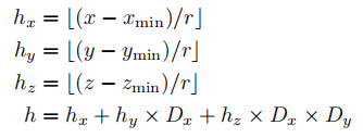
(5) 使用哈希函数将每个点映射到中 ${G_1,G_2,...,G_M}$ 的一个容器 $G_i$ 。
(6) 迭代{G_1,G_2,...,G_M}，得到M个点。

3.2 Results

代码展示

# Open3D: www.open3d.org
# The MIT License (MIT)
# See license file or visit www.open3d.org for details

import numpy as np
from open3d import *

if __name__ == "__main__":

    print("Load a point cloud, print it, and render it")
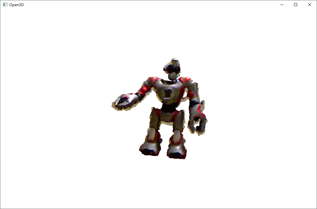
    pcd = open3d.io.read_point_cloud("F:\\guoc\\pointcloud_tutorial-master\\data\\robot1.pcd")
    print(pcd)
    print(np.asarray(pcd.points))
    open3d.visualization.draw_geometries([pcd])

    print("Compute the normals of the downsampled point cloud")
    downpcd = pcd.voxel_down_sample(voxel_size = 0.01)
    downpcd.estimate_normals(search_param = open3d.geometry.KDTreeSearchParamHybrid(
            radius = 0.03, max_nn = 30))
    open3d.visualization.draw_geometries([downpcd])
    print("")

结果展示

原始点云

滤波后的点云

点云兔子

关注

0
点赞
踩
5

收藏

觉得还不错? 一键收藏
打赏
0
评论
Open3d入门

(3)主向量是Ur的列向量。(X的特征向量=H的特征向量)。(6) 迭代{G_1,G_2,...,G_M}，得到M个点。(3)P处的表面法线是PCA的最小特征值对应的特征向量。(1)找到它的K最近的邻居，这些邻居定义了一个表面；对三维点云进行体素网格下采样的方法主要有六个步骤。三维点云的表面法线估计方法主要有三个步骤。(5) 使用哈希函数将每个点映射到中。(4) 计算每个点的体素索引。(2) 确定体素网格大小r。(2)对这些点应用PCA;
复制链接

扫一扫